

[WITH CODE] Data: The criteria you need for market data
Choose data that aligns with your trading strategy and time horizon

Table of contents:
Introduction.
The market data supply chain and data quality criteria.
Quantifying data accuracy.
Assessing granularity.
Latency optimization.
Data completeness and integration.
Matrix-based optimization.
Before you begin, remember that you have an index with the newsletter content organized by clicking on “Read the newsletter index” in this image.

Introduction
Let’s face it: most trading strategies fail not because the math was wrong, but because the data was garbage. Imagine spending weeks building a Ferrari of an algorithm, only to fuel it with yesterday’s lawnmower gas. It’ll sputter, stall, and leave you stranded on the highway of regret.
Choosing data that aligns with your trading strategy and time horizon, while meeting quality, granularity, and low-latency criteria, is crucial for optimizing algorithm performance in dynamic markets.
Let us begin in the world of data-driven algorithmic trading!
The market data supply chain and data quality criteria
The journey of market data from its genesis to its utilization can be broken down into several stages. Each stage adds value and transforms raw data into a more refined product ready for consumption by traders and algorithmic systems.
Exchanges: The primary source of market data, where every tick, trade, and order book update is generated. Here, the data is raw and unprocessed—akin to unrefined ore that must be mined for gold.
Hosting providers & ticker plants: These intermediaries collect data from various exchanges and perform normalization. Normalization standardizes different data formats so that downstream systems can process them uniformly. This stage reduces the engineering burden on quants, who otherwise might need to wrangle disparate data formats.
Feed providers: After normalization, feed providers distribute the data via APIs. These feeds supply real-time or near-real-time market data to traders, thus enabling rapid decision-making in high-speed trading environments.
OMS/EMS software providers: Finally, the data is used by Order Management Systems and Execution Management Systems to assist in executing trades and managing orders. At this stage, the data is processed, user-friendly, and often enriched with additional analytics.
The transformation process can be summarized as:
This journey ensures that the data fed into trading algorithms is accurate, timely, and easily digestible.
But what about the quality? Do we need some kind of criteria?
The answer is yes. Indeed the following criteria must be met:
Accuracy: The data must be free of errors. Mathematically, if we let D represent the dataset and ϵ be the error term, we require
\(\epsilon = 0 \quad \text{or at least} \quad |\epsilon| < \delta\)where δ is a small tolerance level.
Granularity: Data should provide sufficient detail for the strategy. For example, a high-frequency trading algorithm requires tick-level granularity. We can express granularity G in terms of the number of data points per unit time:
\(G=\frac{N}{T}\)where N is the number of data points and T is the time period.
Latency: The delay between data generation and reception must be minimized. If L denotes latency, our goal is to achieve L→0.
Field completeness: The dataset must include all relevant fields—price, volume, bid-ask spreads, etc. We define a completeness vector c where each element represents the availability of a required field:
\(\mathbf{c} \in \{0,1\}^k,\)and we require that the sum of elements equals k—the total number of fields.
Integration and compatibility: The data should integrate smoothly with the trading system’s architecture. This can be modeled as a function I(D,S) that measures the integration quality between data D and system S. Our target is to maximize I.
Most retail traders don't have specific criteria. They drift, settling for whatever's available and free. Even many small and medium-sized firms, at best, purchase data from a recognized data provider, and whatever happens... a little cleaning and off they go!

Quantifying data accuracy
Suppose we have a dataset D consisting of nnn observations. Each observation is represented as a vector di∈Rm, where m is the number of features. The overall dataset can be represented by a matrix:
Let E be the error matrix such that:
where Dtrue is the ideal dataset. The Frobenius norm ||E||F gives a measure of the overall error:
A small value of ||E||F indicates high accuracy. In practical terms, our goal is to have:
If your error norm is larger than your true data norm, you might as well be trading based on random guesses!
Let’s see an example of this.
import numpy as np
import matplotlib.pyplot as plt

def compute_error_norm(D_true, D_candidate):
    """
    Quantifying Data Accuracy

    This snippet computes the Frobenius norm error between a true dataset and candidate datasets
    with varying noise levels. In our paper, we described this metric as:
        ‖E‖₍F₎ = √(Σᵢ Σⱼ (D_candidate - D_true)²)
    which is a key indicator of data accuracy.
    """
    error_matrix = D_candidate - D_true
    return np.linalg.norm(error_matrix, 'fro')

# Simulate a true asset price series (e.g., a linear trend from 100 to 110)
np.random.seed(42)
n_points = 100
true_prices = np.linspace(100, 110, n_points)  # true trend
D_true = true_prices.reshape(n_points, 1)  # shape: (100, 1)

# Evaluate error for candidate datasets with increasing noise
noise_levels = np.linspace(0, 0.5, 20)  # Noise standard deviation from 0 to 0.5
error_norms = []
for noise in noise_levels:
    candidate_prices = true_prices + np.random.normal(0, noise, n_points)
    D_candidate = candidate_prices.reshape(n_points, 1)
    error = compute_error_norm(D_true, D_candidate)
    error_norms.append(error)
The output would be:
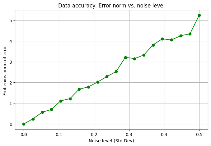
As the noise level increases, the error norm grows, indicating lower data accuracy. This behavior directly reflects our theoretical derivation that higher noise leads to higher error.
Assessing granularity
We already know about the basic ratio of N observations over a period T. This doesn’t require any complex formula. For an algorithm that operates on tick data, a high value of G is essential. If G is too low, the algorithm may miss important microstructure details of the market. To ensure adequate granularity, we can set a minimum threshold Gmin:
Let’s use a toy example to ilustrate this aspect. Using your infra this will change a little bit but I think that it can help to have a general picture.
import numpy as np
import matplotlib.pyplot as plt

"""
Assessing Granularity

In the context of algorithmic trading, granularity (observations per unit time) is crucial.
This snippet simulates trade tick timestamps using an exponential distribution to mimic high-frequency data.
"""

# Simulate trade tick timestamps
np.random.seed(42)
n_ticks = 500  # number of ticks in a trading session
# Assume interarrival times follow an exponential distribution (mean = 0.2 seconds)
interarrival_times = np.random.exponential(scale=0.2, size=n_ticks)
timestamps = np.cumsum(interarrival_times)

# Calculate granularity as the number of ticks per second
total_duration = timestamps[-1] - timestamps[0]
granularity = n_ticks / total_duration
print("Estimated granularity (ticks per second):", granularity)
You would get an histogram like this one:
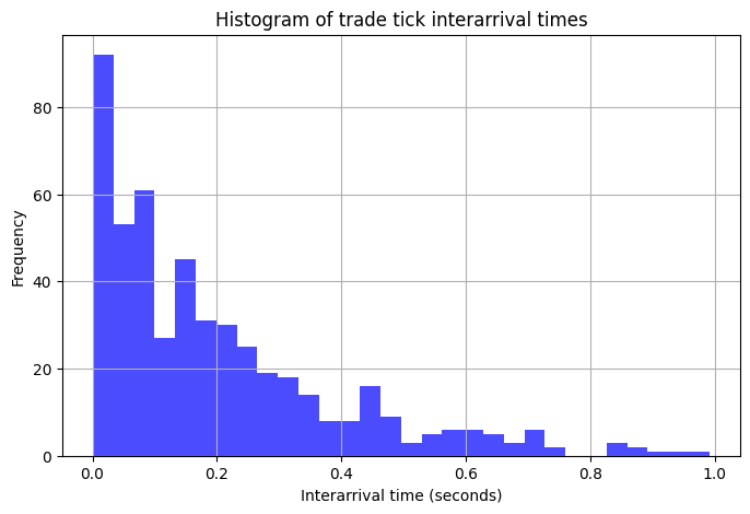
Basically, the histogram shows the distribution of time intervals between trade ticks. The average granularity indicates the data resolution, which is key for capturing market microstructure.
Latency optimization
Latency L is a critical metric in algorithmic trading. If we model the data delivery system as a network with delays, we can use the following expression:
where Δti represents the delay at each stage i of the market data supply chain. The objective is to minimize L such that:
This snippet simulates the impact of decreasing latency on an overall quality score. The quality function aggregates inverse error—accuracy—granularity, inverse latency, and completeness as defined previously.
import numpy as np
import matplotlib.pyplot as plt

def compute_quality(D_true, D_candidate, latency, granularity, completeness, weights):
    """
    Latency Optimization

    This snippet simulates a reduction in data feed latency and evaluates the impact on the overall quality score.
    The quality function used here is:
        Q = w1*(1/‖E‖₍F₎) + w2*G + w3*(1/L) + w4*C
    which highlights the benefit of lower latency.
    """
    eps = 1e-6  # small constant to avoid division by zero
    error_norm = np.linalg.norm(D_candidate - D_true, 'fro')
    q_accuracy = 1 / (error_norm + eps)
    q_latency = 1 / (latency + eps)
    Q = weights[0]*q_accuracy + weights[1]*granularity + weights[2]*q_latency + weights[3]*completeness
    return Q

# Simulate a true asset price series (a slight upward trend)
np.random.seed(42)
n_points = 100
D_true = np.linspace(100, 105, n_points).reshape(n_points, 1)
# Candidate dataset with slight noise
D_candidate = D_true + np.random.normal(0, 0.02, (n_points, 1))

# Set constant granularity and completeness as in our supply chain discussion
granularity = n_points / 1.0  # e.g., 100 ticks per second
completeness = 1.0           # full completeness

# Define weights emphasizing latency (as discussed in our paper)
weights = [0.4, 0.2, 0.3, 0.1]

# Simulate latency reduction (from 50ms to 1ms)
latency_values = np.linspace(0.05, 0.001, 50)
quality_scores = [compute_quality(D_true, D_candidate, lat, granularity, completeness, weights)
                  for lat in latency_values]
Being the output:
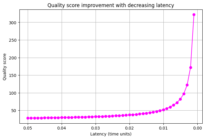
The plot clearly shows that as latency decreases, the quality score improves markedly. The inverse relationship—1/latency—in the quality function underlines the importance of low-latency data feeds.
Data completeness and integration
Let the completeness vector for an observation di be defined as:
where ci,j=1 if field j is present and 0 otherwise. The overall completeness of the dataset is:
A perfect dataset would have C=k. If the integration function I(D,S) is linear with respect to completeness, then we can express:
where α is a scaling factor that depends on system compatibility. Our goal is to maximize I.
This snippet simulates trade record datasets where required fields might be missing. It computes the average completeness ratio and visualizes how it degrades as the probability of missing a field increases.
import numpy as np
import matplotlib.pyplot as plt
import random

def compute_completeness(dataset, required_fields):
    """
    Compute the average completeness ratio for a dataset.
    """
    total_score = 0.0
    for record in dataset:
        present = sum(1 for field in required_fields if field in record)
        total_score += present / len(required_fields)
    return total_score / len(dataset) if dataset else 0

# Define required fields (as per our discussion on data integration)
required_fields = ["price", "volume", "timestamp"]

# Simulate dataset completeness over a range of missing field probabilities
missing_probs = np.linspace(0, 0.9, 10)  # from 0 (all fields present) to 0.9 (high missing probability)
completeness_ratios = []
num_records = 200

for p in missing_probs:
    dataset = []
    for _ in range(num_records):
        record = {}
        # Each required field is included with probability (1 - p)
        if np.random.rand() > p:
            record["price"] = round(random.uniform(100, 150), 2)
        if np.random.rand() > p:
            record["volume"] = random.randint(10, 1000)
        if np.random.rand() > p:
            record["timestamp"] = random.randint(1600000000, 1700000000)
        dataset.append(record)
    completeness_ratios.append(compute_completeness(dataset, required_fields))
The output would be:
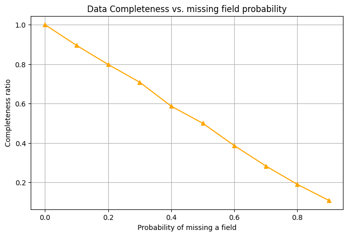
As the probability of missing a field increases, fewer fields are present in each record on average, so the completeness ratio drops. Essentially, the more likely each field is to be missing, the less complete your overall dataset becomes.