Table of contents:
Introduction.
When smoothing data goes too smooth.
Why 1000 decision trees won't let you see the forest.
Feature engineering = Making up fairy tales
Introduction
It’s saturday and you’re at a birthday party. There’s a baby screaming, balloons popping, and your uncle belting out karaoke renditions of “Sweet Caroline.” To drown out the chaos, you put on your noise-canceling headphones and settle in to listen to Mozart. Suddenly, you miss the excitement—a piñata exploding overhead, a wild dance-off, and even a rogue Lego castle that sends your juice box flying.
In algorithmic trading, our market behaves like that screaming baby, full of chaotic noise and unpredictable events. In an effort to cancel out the “noise,” many traders apply sophisticated techniques such as denoising, Random Forests, and feature engineering. However, as we will show, these techniques can lead you astray, much like missing the best parts of the party.
When smoothing data goes too smooth
Let's start from the beginning: What’s denoising?
Donoising is a mathematical process aimed at extracting the underlying signal from a set of noisy observations.
Think of it as using a magic comb to tidy up your dog’s fur. The idea is that by removing the chaotic noise—i.e., the random fluctuations in stock prices—you can reveal a clear pattern that might help forecast future movements.
If we assume that a stock price P(t) can be decomposed as:
Where:
S(t) is the underlying signal, which may contain slow-moving trends and recurrent cycles.
ϵ(t) is the noise, representing short-term volatility and random shocks.
The challenge lies in the fact that, unlike in controlled environments, the distinction between S(t) and ϵ(t) is inherently blurry. An extreme event that appears to be noise might actually be the harbinger of a new trend. Thus, if you employ a denoising technique with a threshold parameter λ:
where D is your denoising operator, you risk filtering out crucial noisy data that contains the seeds of profitable opportunities.
In other words, by setting λ too high, you’re effectively saying, I only want the smooth, boring part of the market, and missing out on the wild swings that sometimes make—or break—a trading strategy.
In many classical approaches, one might employ tools like the Fourier transform or wavelet shrinkage to smooth out this noise. However, when you smooth too much, you risk removing not only the unwanted disturbances but also the important features that indicate profitable trading opportunities.
Imagine a barber who, in trying to give you a neat haircut, accidentally shaves off all your hair! The resulting bald Chihuahua isn’t exactly what you were hoping for. Moreover, these tools are only for labeling. Using them as a sign? It's suicide...
Here one of the classics, the Savitzky-Golay filter from the SciPy library:
import numpy as np
from scipy.signal import savgol_filter
import matplotlib.pyplot as plt
# Generate a fake stock price with a secret signal (sine wave)
t = np.linspace(0, 10, 100)
signal = np.sin(t) * 10 # The "real" pattern
noise = np.random.normal(0, 5, 100) # Chaos (aka market reality)
price = signal + noise
# Denoise it!
denoised = savgol_filter(price, window_length=50, polyorder=2)
# Plotting to visualize the effect
plt.figure(figsize=(10, 5))
plt.plot(t, price, label="Original price (noisy)")
plt.plot(t, denoised, label="Denoised price", linewidth=3)
plt.legend()
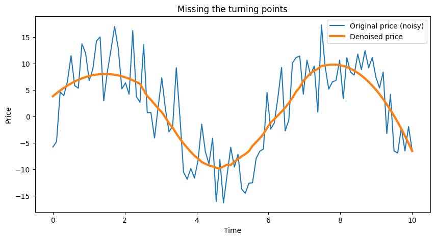
plt.title("Missing the turning points")
plt.xlabel("Time")
plt.ylabel("Price")
plt.show()
In this experiment, the denoised curve looks smooth—almost too smooth. It fails to capture the rapid fluctuations—the turning points—in the actual price, leading to delayed responses in trading decisions.
Essentially, you’re buying late and selling late, and before you know it, your allowance—or trading capital—is evaporating.
But all is not lost, if you are interested take a look at this other version. It is more robust and better than the original filter. All the bugs that Scipy has have been removed. Take a look at my other article:
A more sophisticated approach to denoising employs wavelet transforms. The idea is to decompose the signal into wavelet coefficients and then apply a thresholding operation:
Here:
wk are the wavelet coefficients, representing the strength of the signal at different scales.
ψk are the wavelet functions.
Threshold(wk) sets to zero all coefficients below a certain level.
In markets, rare and extreme events—think of the GameStop saga—manifest as large coefficients. If we threshold these out, we lose the “surprise” factors that often lead to dramatic price movements. It’s like editing out all the explosions from an action movie: you end up with a film about cars discussing tire pressure.
Thus, the very process designed to clarify the picture inadvertently erases critical information, leaving you with a sanitized version of the market that fails to alert you to profitable—or dangerous—anomalies.
Why 1000 decision trees won't let you see the forest
Random Forests are a popular ensemble learning technique in machine learning. The idea is to create a multitude of decision trees, each trained on a random subset of the data, and then aggregate their predictions.
In theory, this approach reduces variance and improves predictive performance. Imagine asking 1000 squirrels to forecast the weather—they might each give you a wildly different answer, but you hope that by averaging their opinions, you’ll get closer to the truth.
In trading, these squirrels—or trees—split the data based on features such as technical indicators or macro data:
Is the RSI above 70? 😬
Did the price eat a burrito yesterday?—Okay, maybe not that one, but you get the idea.
However, the market is not a stationary system. Patterns evolve as quickly as new memes appear on the internet. What worked in one period—say, during a bullish 2022—might completely misfire in the next—a bearish 2023. If your Random Forest is trained on outdated patterns, it becomes a dinosaur predicting tomorrow’s trends using yesterday’s rules.
These rules are aggregated predictions of multiple decision trees that averages the outputs:
This averaging process works well when each tree is an unbiased estimator of the true relationship. However, market dynamics change so rapidly that an estimator trained on past data becomes biased for future conditions.
Below is an illustrative code snippet using scikit-learn’s RandomForestRegressor. It's pretty simple to implement and has so many pitfalls associated with it that it's better not to do it. But anyway, just in case you're curious, here it goes:
from sklearn.ensemble import RandomForestRegressor
import numpy as np
import pandas as pd
# Assume features_2022, price_changes_2022, features_2023 are preloaded Pandas DataFrames/Series
# For the sake of this example, we generate synthetic data
np.random.seed(42)
features_2022 = pd.DataFrame(np.random.rand(100, 5), columns=[f'feature{i}' for i in range(1, 6)])
price_changes_2022 = np.random.rand(100) * 20 - 10 # Simulated percentage changes
features_2023 = pd.DataFrame(np.random.rand(100, 5), columns=[f'feature{i}' for i in range(1, 6)])
# Train a Random Forest model with 1000 trees
model = RandomForestRegressor(n_estimators=1000, random_state=42)
model.fit(features_2022, price_changes_2022)
# Test on new data
predictions = model.predict(features_2023)
print("Predictions for 2023 data:")
print(predictions)
What’s the outcome? The model, having learned patterns from 2022, stubbornly predicts a bullish trend even when the market conditions in 2023 are radically different. It’s like trying to drive using a 1990s map in a modern, constantly changing city—by the time you reach your destination, the roads have all shifted.
If you really want to use this model, you should build it sequentially—but for time series this is also a bad idea, check it here: [Link]. Personally, I like the incremental version where training is online, without partitions between train and test, but we can leave this for a future post.
Random Forests build on the idea of minimizing a metric called Gini impurity—or sometimes entropy—at each split. For a given feature Xj, the algorithm searches for a split point sss that maximizes the information gain:
Where:
Iparent is the impurity of the parent node.
Ileft and Iright are the impurities of the left and right child nodes.
Nleft and Nright are the number of samples in these nodes.
N is the total number of samples.
In a static dataset, this metric helps build a robust tree. But in the market, today’s information gain can be tomorrow’s information garbage. Even if a split seems optimal at the moment, the rapid evolution of market conditions can render that decision obsolete almost instantly. You’re essentially using a perfectly good pizza cutter to slice water—an exercise in futility that leaves you with nothing but soggy disappointment.
Feature engineering = Making up fairy tales
Feature engineering is the art of creating new input variables—aka features—that might help your model discover hidden patterns. For instance, you might calculate:
The 10-day moving average of volume divided by the open price.
The number of times the CEO posted on tusdays during the earnings release.
While these features may sound intriguing—or downright silly—they often represent arbitrary transformations of the raw data. The underlying assumption is that by crafting these novel features, you’re providing the algorithm with magical insights into the market’s behavior.
However, here’s the kicker: every extra feature increases the chance of fitting your model to randomness rather than genuine signal. It’s like a storyteller who adds more and more details until the original plot is completely lost in a sea of irrelevant subplots.
You may end up with a tale so convoluted that even the intended message disappears in the noise—resulting in decisions that lead to financial losses. Note the playful absurdity of some of these transformations:
import pandas as pd
import numpy as np
# Generate synthetic market data
data = pd.DataFrame({
'volume': np.random.randint(100, 1000, 100),
'price': np.random.rand(100) * 100,
'high': np.random.rand(100) * 105,
'low': np.random.rand(100) * 95
})
# Invent 100 "awesome" features
X = pd.DataFrame()
X["feature1"] = data["volume"].rolling(10).mean() / np.cos(data["price"])
X["feature2"] = data["high"] * data["low"] + data["volume"].diff(2)
# ... Imagine 98 more nonsensical features ...
# For demonstration, we simulate target values
y = data["price"].diff().fillna(0)
# A dummy model training (this is just for illustration)
from sklearn.linear_model import LinearRegression
model = LinearRegression()
model.fit(X.fillna(0), y)
print("Model score:", model.score(X.fillna(0), y))
This useless feature factory churns out features that are more like imaginative fables than statistically meaningful predictors. When you train a model on these features, it might give you an accuracy score that makes no sense.
Indeed, in our example and depending on the seed, the score might even be negative—a clear sign that the model is not just wrong, but cheerfully off the mark. But for the sake of this article, we are expanding this section a little further to have a complete overview.
To give you an idea, the standard pipeline any quant follows is based on:
Besides, feature engineering involves applying a transformation function ϕ to the original data X:
The Johnson-Lindenstrauss lemma provides a reminder that when data is projected into high-dimensional spaces, distances can become distorted:
for all vectors u and v in the original space, where ϵ is a small constant.
As you add more features, the distance between data points may not represent any meaningful relationship. Instead, every new feature could be mistaken for a genuine signal. It’s like inflating a balloon with too much air—what seemed clever at first becomes a fragile, overblown bubble ready to burst.
The danger is that your model becomes enamored with these spurious patterns, leading to trading decisions that are based on fancy math rather than market reality. In the end, you’re left chasing shadows, while the market—ever unpredictable—carries on like a mischievous storyteller.
At this point in our artcile, you might be wondering: If denoising, Random Forests, and feature engineering can all lead to disaster, what should I do? We will see the answer in future articles.
Until next time—may your code compile on the first try, your FPGA stays frosty, and your predictions always land right on target! 👨💻
👍 Did you gain valuable insights and now want to empower others in the field?
Appendix
Sequential Boosting for Learning a Random Forest [Paper]
On-line Random Forest [Paper]
Sequential Feature Selection [Paper]