

[WITH CODE] Risk Engine: Capital allocation
How much capital should be allocated to each strategy?

Table of contens:
Introduction.
Risk identification and dilemmas.
The mathematical architecture of AO.
Principled regularization.
Synergistic learning.
Adaptive aggregation.
The system selection.
Conformal calibration for credible intervals.
Before you begin, remember that you have an index with the newsletter content organized by clicking on “Read full story” in this image.

Introduction
We’re all chasing alpha, but let’s be honest—most models fail because they’re built on shaky assumptions. You know the drill: overfitting historical data, blowing up when regimes shift, or acting like inscrutable black boxes. It’s like trying to predict tomorrow’s weather using yesterday’s forecast and a broken barometer.
Here’s the reality check. A single god system won’t save you. Markets aren’t static; they’re a shape-shifting puzzle. Simple model averaging? That’s just throwing spaghetti at the wall and hoping something sticks. What we need are multiple systems.
Take overfitting. We’ve all been there—your strategy crushes in-sample data, then flops live. Why? Because it’s memorizing noise, not learning signals. And regime shifts? Even the smartest models get caught flat-footed when correlations flip overnight—looking at you, 2008 and 2020. Then there’s the black box problem: if you can’t explain why your model makes a decision, how do you troubleshoot when it goes rogue?
The answer isn’t more complexity—it’s smarter structure. Instead of one monolithic algorithm, you build a team of specialized predictors—each one for different market regimes, asset behaviors, or risk factors. Then, you dynamically weight their outputs using techniques like kernel-based aggregation, which adapts to changing conditions.
But here’s the kicker: uncertainty quantification. If your model says “S&P up 1% tomorrow,” but doesn’t tell you the confidence level, you’re flying blind. Today’s framework bakes in probabilistic outputs. That way, trading isn’t a guessing game; it’s data-driven.
As you already know, alpha isn’t about beating the market on day one. It’s about building systems that survive day 100.

Risk identification and dilemmas
Algorithmic trading systems face an inherent paradox: they must be responsive enough to capture genuine market movements yet stable enough to ignore random noise.
This dual requirement creates a statistical tension that conventional models struggle to resolve. Single-model approaches typically excel in one domain but falter in the other—either reacting too quickly to market changes—overtrading—or too slowly—missing opportunities.
Consider the trader's dilemma: when do multiple weak signals combine to form a reliable trading thesis, and when are they merely echoing the same underlying noise?
The mathematical question becomes: how can we optimally aggregate information across diverse predictive models, each with its own strengths and weaknesses?
The Aggregation Opt model (AO) encounters several intrinsic risks that warrant careful consideration:
The AO model's performance critically depends on its systems’ performance selection mechanism. Poor selection creates a cascading effect of suboptimal predictions aka bias selection.
The dual-stage modeling approach—base learners followed by aggregation—introduces multiple opportunities for overfitting, potentially leading to catastrophic performance degradation in production.
The conformal prediction component can fail during abrupt losses because some models are correlated and deviate.
With numerous tunable parameters—mixing rate, ridge penalties, kernel bandwidth—the model risks becoming excessively sensitive to hyperparameter choices.
The breakthrough in addressing these challenges emerged from a pivotal conceptual shift:
The realization that systems shouldn't merely be averaged but structurally integrated through their statistical relationships. This shift transformed ensemble methods from simple averaging mechanisms to structured learning frameworks.
The pivotal insight was that systems contain information not just in their outputs but in their error structures. When two systems make similar mistakes, they likely capture similar market dynamics. This correlation structure itself becomes valuable information that can be leveraged through kernel methods to achieve better aggregation.
This revelation forms the foundation of the AO, which systematically exploits these statistical relationships to create a prediction framework that is simultaneously robust to noise and responsive to genuine market signals.

The mathematical architecture of AO
Believe it or not, the AO is a system that was born from an insane argument on Linkedin. It distinguishes itself from the ideas of other quants because it seeks to lay the foundation stone for a risk framework. The first step is knowing how much capital to allocate to a portfolio of systems. In fact, leaving aside the pricing aspect, the three basic pillars would create it:
Capital allocation.
Number of contracts.
Inventory management.
This architecture represents a deliberate departure from conventional methods, introducing structured dependencies between component models. We'll develop this in the coming days or weeks. For now, let's focus on today's point, which answers the question: How much capital do I invest in a system?
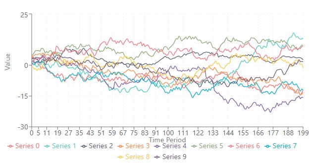
Imagine these are the performances of your systems. Some are fucking garbage, and others perform reasonably well, depending on when they operate, who we give money to, and how much.
The mathematical core consists of three interrelated components:
A collection of regularized linear techniques that capture different aspects of systems behavior.
A non-linear weighting mechanism that leverages similarities between prediction patterns.
A distribution-free approach to constructing valid prediction intervals.
These components work in concert to create a prediction framework that balances accuracy, stability, and uncertainty quantification.
Principled regularization
The siren song of overfitting is perhaps the most persistent peril in quantitative finance. A model that perfectly explains past market movements often does so by memorizing noise, not by learning genuine underlying signals. When faced with new, unseen data, such a model falters, often catastrophically.
How do we build base learners–our individual predictive units–that are robust and generalize well?
The answer lies in Ridge Regression, a technique that acts as a disciplined overseer.
You can go deeper by checking this document:
It allows this method to learn from the data but penalizes excessive complexity in the learned parameters—weights. Think of it as building a skyscraper: you need a foundation that can withstand tremors, not one built on shifting sands. Ridge regression provides this stability.
Ridge Regression seeks to find the weight vector that minimizes the sum of squared errors plus a penalty term:
A larger α imposes a greater penalty on large weights, effectively shrinking them and preventing any single feature from having an outsized influence. This leads to smoother, less complex models that are less prone to latching onto spurious patterns.
The solution to this optimization problem is given by the normal equations:
where Ip is the p×p identity matrix.
To solve this efficiently, it employs Cholesky factorization. We decompose
into LLT, where L is a lower triangular matrix. Then, we solve Lz=XTy for z—forward substitution—and subsequently LTw=z for w—backward substitution.
The _solve_ridge method in our Python class encapsulates this vital step:
def _solve_ridge(self, X: np.ndarray, y: np.ndarray) -> np.ndarray:
        """
        Solve (X^T X + alpha I) w = X^T y with Cholesky for efficiency.
        """
        n_features = X.shape[1]
        A = X.T @ X + self.ridge_alpha * np.eye(n_features) # Form A
        L = np.linalg.cholesky(A)                           # Cholesky decomposition
        b = X.T @ y
        z = np.linalg.solve(L, b)                           # Solve Lz = b
        return np.linalg.solve(L.T, z)                      # Solve L^T w = z
This robust foundation ensures that each base learner, trained for different aspects of our selected systems, begins its life with a degree of inherent stability, guarding against the treacherous currents of overfitting.
Synergistic learning