[WITH CODE] RiskOps: Exit policy and exit rules

Embrace a proactive approach to exit trades and anticipate market reversals, safeguard your investments, and convert potential pitfalls into opportunities

---

Table of contents:

1. Introduction.

2. What is an exit policy?

3. Next level of concretion, exit rule.

4. The exit strategy as a tactical approach.

---

Introduction

Entries are like fireworks that light up the sky. Everyone loves the sparkle and the thrill of those moments when you jump into a trade, expecting your portfolio to shoot to the moon. Everyone loves talking about entries—those flashy moments when you jump into a trade like a superhero.

But what about exits? Exits are like Batman—the thoughtful, well-planned decisions that prevent catastrophic losses and help secure profits. Think of exits as the afterparty cleanup crew: they ensure that all the excitement doesn't end in a financial mess.

In my view, modeling the exit of a trade is by far the most important thing to do when putting money at risk. The so vilified, forgotten, and misunderstood exits... Generally, we find two cases:

• The quants focused on modeling the entry signal and finding a miracle variable that allows them to predict something and justify their salary.

• The retail amateur—in the best-case scenario—setting a tight stop-loss at the entry point, basically anywhere and in any way.

Now, there are 3 fundamental levels to keep in mind: Policy → Rule → Strategy

What is an exit policy?

An exit policy is the overarching rulebook that helps you decide how much you’re willing to risk on a trade. Much like your parents set limits on your allowance or screen time, exit policies set the boundaries for how much money can be lost in any single trade. This is your risk management blueprint, designed to keep your portfolio from being devoured by the wild beasts of the market.

Basically, it is like the constitution of your trading system. It sets the overarching guidelines that govern all your trades. Think of it as the rules of the game, ensuring that no single trade can sink your entire portfolio. It is a strategic safeguard designed to:

1. Set strict loss limits, the policy ensures that even during adverse market conditions, your overall capital is protected.

2. Minimize emotional decisions, ensuring consistency and adherence to your trading plan.

3. Allow you to manage trades of various sizes without compromising the overall health of your portfolio.

A robust exit policy typically includes the following core components:

• Risk caps: No single trade should result in a loss exceeding 2% of the entire portfolio value.

• Stop-loss mandates: Every trade must have a stop-loss order.

• Daily loss limits: The total daily loss per trading strategy should not exceed 5% of the allocated capital.

To illustrate why this is important, let’s consider a simple portfolio with an initial value P₀​. If a trade results in a loss L, then the remaining portfolio value P after the trade is given by:

\(P=P_0-L\)

To ensure no single trade exceeds 2% of the portfolio value, we set:

\(L \leq 0.02 \times P_0 \)

This ensures that even if the worst happens, your portfolio remains stable.

This is what would happen if you have a streak where you only lose and you go without the brakes of the 2%

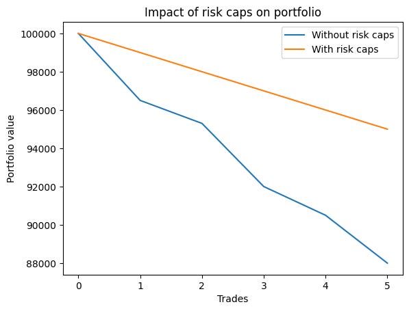
Simply, crazy. As you can see, risk caps act as a safety net, preventing catastrophic losses.

But here the issue, how to coordinate those three? Let's develop it step by step.

1. Per-trade risk management with stop-loss orders:

   For each trade i:

   • Determine the maximum allowable dollar loss:

     \(R_i^{\text{max}} = 0.02 \times P\)

   • Set the stop-loss order based on your entry price E_i​ and your chosen stop-loss percentage δ_i:

     \(S_i = E_i \times (1 - \delta_i)\)

   • Size your position—number of shares or units, N_i​—so that the potential loss does not exceed the maximum allowable dollar loss:

     \(N_i \leq \frac{0.02 \times P}{E_i \times \delta_i}\)

   This ensures that if the trade moves against you and hits the stop-loss price, the loss will be capped at 2% of your portfolio.

2. Daily loss aggregation:

   Even if every individual trade is capped at 2% loss, multiple trades in a single day could collectively exceed your daily risk limit. Suppose you execute nnn trades in one day, then the sum of losses must satisfy:

   \(\sum_{i=1}^{n} L_i \leq 0.05 \times P\)

   For instance, if you take three trades in a day, even if each is allowed up to 2% loss, the maximum theoretical total loss would be:

   \(3 \times 0.02 \times P\)

   which would exceed the 5% daily limit. Therefore, you must manage the number of trades or adjust position sizes such that the aggregated risk remains within the daily cap.

   One practical approach is to set a rule like:

   • Only execute a new trade if the cumulative loss for the day plus the risk of the new trade is less than or equal to 5% of P:

     \(\left( \sum_{i=1}^{k} L_i \right) + \left( E_{k+1} \times \delta_{k+1} \times N_{k+1} \right) \leq 0.05 \times P \)

     where k is the number of trades already taken that day.

Okay! Time to move to the next level.

Next level of concretion, exit rule

Now that we’ve established the big picture, let’s zoom in on the specifics. If exit policies are like your parent’s overall guidelines, then exit rules are the sharp looks your mom gives you when you’re about to sneak a cookie after bedtime.

Exit rules are the actionable instructions that tell your trading algorithm exactly when to pull the plug. These rules are precise and programmable, often based on price movements or other variables.

The most basic examples are:

• Fixed percentage stop-loss: Close the position if the asset price falls by 3% from the purchase price.

• Trailing stop-loss each N points: Allow the stop price to increase as the asset price increases but never decrease below a certain percentage of the peak price—N points is the part that belongs to the exit rule while the trailing stop-loss is part of the exit strategy.

Let's start with the first one, a fixed percentage. Consider you have purchased a stock at an entry price E. An exit rule might specify that if the stock price falls by 3% from the entry price, it’s time to exit. The stop-loss price S is then given by:

\(S = E \times (1 - 0.03) \)

For an entry price of $50, this becomes:

\(S = 50 \times (1 - 0.03) = 50 \times 0.97 = \$48.50 \)

So, if the stock price hits $48.50, you should exit the trade. The formula for the stop-loss price can be understood by considering a percentage decrease. A 3% decrease means that only 97% of the original price remains. In more general terms, if the percentage decrease is δ, then the stop-loss price S is:

\(S = E \times (1 - \delta) \)

For δ=0.03, we have:

\(S = E \times 0.97 \)

This simple multiplication encapsulates the idea of preserving capital by capping losses. May this is the easiest way:

# Define the entry price and the stop-loss percentage
entry_price = 50  
stop_loss_percent = 0.03  

# Calculate the stop-loss price
stop_price = entry_price * (1 - stop_loss_percent)

# Let's simulate a scenario where the current price is at the stop-loss level
current_price = 48.50  # Uh-oh!

if current_price <= stop_price:
    print("Abandon ship!!")

n contrast to fixed stop-losses, trailing stop-losses offer a dynamic approach that adapts as the asset’s price moves favorably. Imagine buying an asset at price P_buy​. and setting a trailing stop-loss at T%. As the asset price increases, the stop-loss price P_stop​ is recalculated to lock in gains, while it never moves lower than a preset percentage below the peak price:

\(P_{\text{stop}} = \max \left( P_{\text{stop}}, (1 - T) \times P_{\text{current}} \right) \)

Where P_current is the current price of the asset.

This rule ensures that if the market reverses, you secure your profits by exiting at the highest possible price within the safety range.

Let' use a simulation for that:

import numpy as np

# Simulated price data
prices = np.array([100, 105, 110, 115, 120, 118, 116, 114, 112, 110])

# Calculate trailing stop-loss prices
trailing_percentage = 0.05
stop_loss_prices = []
stop_loss = (1 - trailing_percentage) * prices[0]
for price in prices:
    stop_loss = max(stop_loss, (1 - trailing_percentage) * price)
    stop_loss_prices.append(stop_loss)

# Plotting
plt.plot(prices, label="Asset price")
plt.plot(stop_loss_prices, label="Trailing stop-loss")
plt.xlabel("Time")
plt.ylabel("Price")
plt.title("Trailing stop-loss in action")
plt.legend()
plt.show()

The resulting plot visually demonstrates how the trailing stop-loss adjusts upward as the asset price increases, effectively "trailing" the price while ensuring that profits are protected in case of a downturn.

Now that we have understood exit policies and the precise exit rules with a concrete example, we naturally progress to crafting comprehensive exit strategies. In the next section, we will blend these ideas into dynamic strategies that adapt as the market changes.

The exit strategy as a tactical approach

Finally, we arrive at the tactical level: the exit strategy. This is where the rubber meets the road. An exit strategy considers how all the pieces fit together, optimizing the interaction between entry signals, profit targets, and market conditions.

It is like the conductor of an orchestra, blending the rigid structure of policies with the rapid responsiveness of rules. It’s a master plan that not only protects your capital but also ensures you capture gains when the market is in your favor.

Most common types of exit strategies:

• Pre-set exit targets: Clear price points where profits are realized and positions are closed.

• Market sentiment-based exit: Use sentiment analysis to decide when to exit.

• Trailing stop-loss: As discussed, to dynamically protect gains as the market moves favorably.

• Time-based exit: Predefined durations after which a trade is closed, irrespective of its performance, to mitigate exposure to prolonged market uncertainty.

This blend of rules ensures that your strategy is not rigid but adaptive, allowing you to respond quickly to changing market conditions while sticking to the client profile—if you have any.

For traders who employ quantitative methods, optimizing the balance between risk and return can be formalized using a utility function. You could use a utility function U that balances these two factors:

\(U = \alpha \times R - \beta \times V \)

Where:

• R is the expected return.

• V is the variance—a measure of risk.

• α and β are weights reflecting your risk tolerance and risk/reward preferences.

We want to maximize this utility function to find the optimal θ. And because optimization routines typically minimize a function, we instead minimize:

\(\text{Loss}(\theta) = -U(\theta) \)

One way to optimize this function is by using numerical methods, as illustrated below—remember that this is a toy example.

import numpy as np
import matplotlib.pyplot as plt
from scipy.optimize import minimize

def simulate_trade(prices, theta):
    """
    Simulate a trade using a provided array of prices and a trailing stop-loss parameter theta.
    
    Parameters:
    - prices: Array of prices over time for a single trade.
    - theta: Trailing stop-loss percentage (e.g., 0.05 for 5%).
    
    Returns:
    - exit_price: The price at which the trade is exited.
    - exit_index: The index at which the trade is exited.
    """
    entry_price = prices[0]
    peak = entry_price
    exit_price = prices[-1]  # Default: exit at the last price if stop never triggered.
    exit_index = len(prices) - 1

    for i, price in enumerate(prices):
        # Update peak price if current price is higher.
        if price > peak:
            peak = price
        # If current price falls below the trailing stop-loss threshold from the peak, exit.
        if price < (1 - theta) * peak:
            exit_price = price
            exit_index = i
            break
            
    return exit_price, exit_index

def evaluate_theta(theta, prices):
    """
    Evaluate the performance of a given theta using a single price array.
    
    Parameters:
    - theta: Trailing stop-loss parameter.
    - prices: Array of prices representing one trade.
    
    Returns:
    - trade_return: The percentage return for the trade.
    """
    exit_price, _ = simulate_trade(prices, theta)
    trade_return = (exit_price / prices[0]) - 1
    return trade_return

# Define a single array of prices (historical data for one trade session)
prices = np.array([100, 102, 104, 107, 105, 103, 101, 100.5, 100, 99])

# Set risk/reward preference weights.
# With one trade, we focus on maximizing return.
alpha = 1  # Weight for return.
beta = 0   # No penalty for variance here.

def utility(theta, prices, alpha, beta):
    """
    Utility function for a single trade.
    Since we only have one trade, we aim to maximize the return.
    (Variance is omitted or set to zero.)
    
    Parameters:
    - theta: Strategy parameter (trailing stop-loss percentage).
    - prices: Array of prices.
    - alpha: Weight for returns.
    - beta: Weight for risk (variance), not used here.
    
    Returns:
    - Negative utility (for minimization).
    """
    trade_return = evaluate_theta(theta[0], prices)
    # Utility is just the weighted return here.
    utility_value = alpha * trade_return
    return -utility_value  # Negated for minimization

# Initial guess for theta (e.g., 5% trailing stop-loss)
theta_initial = [0.05]
# Set bounds for theta, for example, between 1% and 10%
bounds = [(0.01, 0.1)]

# Optimize the utility function to find the best theta
result = minimize(utility, theta_initial, args=(prices, alpha, beta), bounds=bounds)
optimal_theta = result.x[0]

print("Optimal trailing stop-loss (theta):", optimal_theta)

# Visualization: Plot the price series and the trailing stop-loss line using the optimal theta.
exit_price, exit_index = simulate_trade(prices, optimal_theta)
peak = prices[0]
trailing_stop = []
for price in prices:
    if price > peak:
        peak = price
    trailing_stop.append((1 - optimal_theta) * peak)

plt.figure(figsize=(8, 4))
plt.plot(prices, marker='o', label="Price")
plt.plot(trailing_stop, linestyle='--', label="Trailing stop-loss")
plt.axvline(x=exit_index, color='red', linestyle='--', label="Exit point")
plt.xlabel("Time step")
plt.ylabel("Price")
plt.title("Trade simulation with optimal trailing stop-loss")
plt.legend()
plt.show()

This plot shows the price path, the dynamically adjusted trailing stop-loss line, and the exit point where the stop-loss was triggered.

This function uses a price array to simulate the trade. It updates the peak price as it moves through the array and exits when the current price falls below (1−θ)×peak.

Most of my systems use:

• Time-based exits.

• Exits based on conditions inherent to market transactions.

• Scale out.

• Volatility-adjusted exists.

Whatever you choose must be consistent with the underlying architecture of the system.

Alright traders, until next time—may your signals be crisp, your execution flawless, and your alpha remain a mystery to the crowd! 🚀

PS: Following the survey from the other day, I would like to ask you what you think about a platform that gives signals based on news. In other words, they would be systems based on volatility, which is where the party is. Let me know in the comments what you think about that. Would you use it?

---

👍 Who do you know who is interested in quantitative finance and investing?

---

Appendix

If you like this topics may you are interested in this two books:

• Risk Management in Trading by John C. Hull.

• Mathematics for Finance: An Introduction to Financial Engineering by Tomasz Zastawniak.