

RiskOps: Traditional sizing methods
Why ‘go big or go home’ is a lie—and how to play the long game with surgical precision

Table of contents:
Introduction.
Sizing based on fixed fractional.
Sizing based on volatility targeting
Sizing based on Monte Carlo simulations.
Sizing based on Omega ratio.
Bonus: Theoretical foundations of conformal prediction in contract sizing.
Before you begin, remember that you have an index with the newsletter content organized by clicking on “Read full story” in this image.

Introduction
Everyone knows the typical trader who is 99% sure that their algorithm will win—until the account burns. They bet everything on that certainty. Then the market slips through his fingers like sand —hello, unexpected news!—and, poof, their money is gone.
Confidence is like a shiny balloon: fun until it pops, leaving you with a bunch of deflated dreams. Risk management, on the other hand, is the string that keeps the balloon from drifting away.
In trading, if you use mediocre models, it’s not enough to have a good prediction; you need to size your positions based on quantifiable risk. Now, if you drink from the Holy Grail, ahhh! Brother, equiponderate is God.
Let’s start with the simplest risk rule: fixed fractional sizing. Think of it as the “fuel gauge” method—where your trading algorithm only burns a measured amount of capital on each trade, ensuring you never run out of fuel on your journey, no matter how strong the signal.

Sizing based on fixed fractional
Imagine your algorithm is like a sophisticated trading system that generates signals for when to enter a trade. These signals might be as tempting as an all-in recommendation from your favorite robo-advisor. However, even if the algorithm is screaming, this stock is going to skyrocket!, your system must still follow a disciplined approach to avoid catastrophic losses.
Instead of diving in headfirst and allocating all your capital based solely on a strong signal, you treat your available capital like the fuel in your algorithm’s trading engine. You only commit a fixed fraction of that fuel per trade. This is analogous to a well-designed trading system that never burns through its reserves by risking only a predetermined percentage of capital on any single trade.
Assume your total capital is C dollars, and you decide to risk a fixed percentage rf on every trade. Then your risk per trade—in dollars—is:
Now, suppose you buy an asset at a price Pentry and set a stop loss at a relative distance δ—e.g., 10%. The potential loss per share is then:
If you buy N shares, the total loss if the stop is hit is:
To ensure that your loss does not exceed your predetermined risk dollars, set:
which rearranges to give:
This simple equation guarantees that you only risk a small, fixed percentage of your capital on each trade—regardless of your algorithm’s level of confidence.
Let’s implement it with a plot that shows how the number of shares changes as the stop-loss distance increases.
import numpy as np
import matplotlib.pyplot as plt
def fixed_fractional(capital, risk_percent=0.02, stop_loss=0.10, entry_price=100):
"""
Calculate the number of shares to buy using fixed fractional sizing.
Parameters:
capital (float): Total capital available.
risk_percent (float): Fraction of capital to risk per trade.
stop_loss (float): Stop-loss distance as a fraction of the entry price.
entry_price (float): Price at which the asset is bought.
Returns:
float: Number of shares to buy.
"""
risk_dollars = capital * risk_percent
return risk_dollars / (entry_price * stop_loss)
# Let's test this
capital = 1000
shares = fixed_fractional(capital, risk_percent=0.02, stop_loss=0.10, entry_price=50)
print(f"Buy {shares:.2f} shares.")
# Effect of stop_loss on the number of shares
stop_loss_range = np.linspace(0.01, 0.20, 100)
N_values = [fixed_fractional(capital, risk_percent=0.02, stop_loss=sl, entry_price=50) for sl in stop_loss_range]
plt.figure(figsize=(8, 4))
plt.plot(stop_loss_range, N_values, label='Shares (N)', color='darkblue', linewidth=2)
plt.xlabel("Stop-Loss distance (δ)")
plt.ylabel("Number of shares (N)")
plt.title("Fixed fractional sizing: N vs. Stoploss distance")
plt.legend()
plt.grid(True)
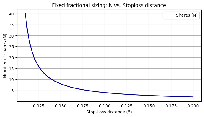
plt.show()This plot shows the amount of shares vs. stop-loss distance. Wider stops = fewer shares. It’s like filling fewer cups if you pour lemonade into bigger mugs.
With fixed fractional sizing locking down basic risk, we now move on to a method that adapts to market mood swings—volatility targeting.
Sizing based on volatility targeting
When the market is calm, prices move gently; when it’s wild, prices swing like needles. Volatility, denoted by σ quantifies this unpredictability. Volatility targeting adjusts your position size based on market volatility to keep your risk constant.
Let’s say your risk budget for a trade is R dollars. High σ = needles mode. To ensure that your exposure remains consistent, regardless of volatility, you set:
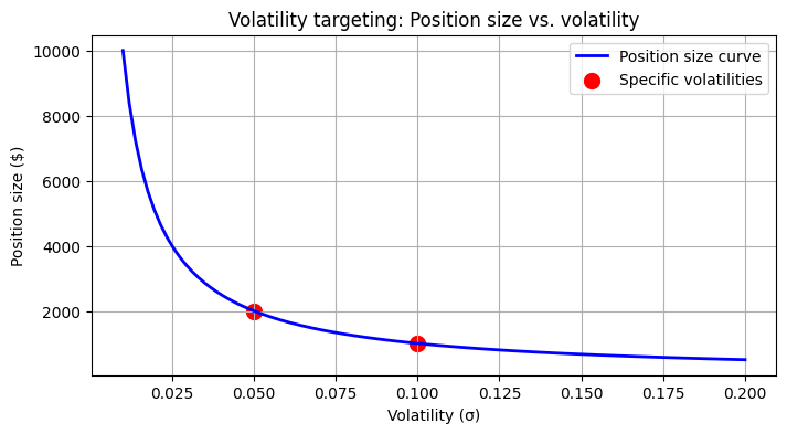
For example, if your risk budget is $100 and the volatility is 5%—σ=0.05—then your position size is:
If volatility doubles to 10%—σ=0.10—the position size halves:
This inverse relationship ensures that when the market becomes more uncertain, you reduce your exposure, protecting your capital.
Let's get our hands on that code!
import numpy as np
import matplotlib.pyplot as plt

def volatility_target(risk_budget, volatility):
    """
    Compute the position size based on volatility targeting.

    Parameters:
        risk_budget (float): Dollar amount you are willing to risk.
        volatility (float): Standard deviation (σ) of returns.

    Returns:
        float: Position size in dollars.
    """
    return risk_budget / volatility

risk_budget = 100
vol_low = 0.05  # 5% volatility
vol_high = 0.10 # 10% volatility
pos_size_low = volatility_target(risk_budget, vol_low)
pos_size_high = volatility_target(risk_budget, vol_high)
print(f"Position size at 5% volatility: ${pos_size_low:.0f}")
print(f"Position size at 10% volatility: ${pos_size_high:.0f}")

# Plot
vol_range = np.linspace(0.01, 0.20, 100)
pos_sizes = [volatility_target(risk_budget, vol) for vol in vol_range]
plt.figure(figsize=(8, 4))
plt.plot(vol_range, pos_sizes, 'b-', label='Position size curve', linewidth=2)
plt.scatter([vol_low, vol_high], [pos_size_low, pos_size_high], color='red', s=100, label='Specific volatilities')
plt.xlabel("Volatility (σ)")
plt.ylabel("Position size ($)")
plt.title("Volatility targeting: Position size vs. volatility")
plt.legend()
plt.grid(True)
plt.show()
Position size plunges as volatility spikes—like shrinking your surfboard when waves get huge:
With volatility captured mathematically, we now turn our attention to simulation-based methods—Monte Carlo simulations—that help us prepare for extreme market events.
Sizing based on Monte Carlo simulations
The markets can be unpredictable—sometimes behaving like a drunken robot with a PhD in uncertainty. Monte Carlo simulations allow us to model thousands—or even millions—of potential future scenarios using stochastic processes. A common model is the geometric Brownian motion, defined by the stochastic differential equation:
where μ is the drift—expected return—σ is the volatility, and Wt is a Wiener process representing the random movement. When integrated, the solution is:
By simulating many paths Pt, we estimate the distribution of future prices—and, importantly, the worst-case loss. If we choose a confidence level α—say, 95%—then we define Lworst as the loss corresponding to the (1−α) percentile. Our position size multiplier is then:
where R is the risk budget.
While GBM assumes normally distributed returns, real markets often show skewness—asymmetry—and kurtosis—fat tails. These properties mean that extreme events happen more frequently than a normal distribution predicts.
Mathematical considerations [In depth]