

[WITH CODE] Risk Engine: Adaptive bailout system
Implementing adaptive systems that detect unexpected anomalies and protect trading performance

Table of contents:
Introduction.
Calibrated risk.
Adaptive bail out.
Before you begin, remember that you have an index with the newsletter content organized by clicking on “Read full story” in this image.

Introduction
Algorithmic trading isn’t for everyone—it takes grit and adaptability. While conformal prediction’s basics are familiar—I’ve covered them before—this time we’re tackling something new: reinventing how these concepts protect trading algorithms. Our mission for today? Designing smarter bailout systems that spot weird market activity on the fly.
Think of your trading algorithm like a stunt pilot. Right now, most systems use rigid safety rules—like a parachute that only deploys at a fixed altitude. But what if, instead, the pilot’s gear could sense turbulence mid-flight and adjust the harness in real time? That’s the vision here: a bailout system that learns as it goes, spots sudden market shifts, and still stays rooted in conformal prediction’s no-nonsense, data-agnostic math.
We’ll skip the basics. For more check here:

And for other application, check the paper Theorical Foundations of Comformal Prediction in Contract Sizing. Available here:
In what follows, we focus on two core concepts:
Calibrated risk: Leveraging a sliding window of recent observations, this component computes prediction intervals that mirror the current error distribution.
Adaptive bail out: This mechanism measures deviations between observed values and prediction intervals, triggering an intervention when those deviations exceed a dynamic threshold linked to market volatility.
Bottom line? It’s about building algorithms that don’t just survive market madness—they sense it coming.
Calibrated risk
For a new observation xnew, our regression model provides a prediction
We maintain a calibration set
and compute the nonconformity scores for each calibration point as
Then, the quantile threshold q is defined as the (1−ϵ)-quantile of these scores:
The adaptive prediction interval for xnew is then given by:
These computations are performed dynamically as new calibration data are added. The sliding window mechanism ensures that only the most recent N data points are used so that the calibration set reflects current market conditions.
To go deeper, check this:
Let’s see how to implement it:
import numpy as np

# Dummy regression model.
class DummyModel:
    def predict(self, X):
        # For simplicity, our model returns the first feature as the prediction.
        return np.array([x[0] for x in X])

# Adaptive Conformal Predictor class.
class AdaptiveConformalPredictor:
    def __init__(self, model, epsilon=0.05, window_size=100):
        """
        Adaptive conformal predictor that updates calibration dynamically.

        Parameters:
        - model: a regression model with a .predict() method.
        - epsilon: initial significance level.
        - window_size: number of recent points for calibration.
        """
        self.model = model
        self.epsilon = epsilon
        self.window_size = window_size
        self.calibration_X = None
        self.calibration_y = None
        self.nonconformity_scores = None

    def update_calibration(self, X_new, y_new):
        """
        Update calibration data with new observations.

        Parameters:
        - X_new: new feature observations.
        - y_new: new target values.
        """
        if self.calibration_X is None:
            self.calibration_X = X_new
            self.calibration_y = y_new
        else:
            self.calibration_X = np.vstack([self.calibration_X, X_new])
            self.calibration_y = np.concatenate([self.calibration_y, y_new])

        # Retain only the most recent window_size points.
        if len(self.calibration_y) > self.window_size:
            self.calibration_X = self.calibration_X[-self.window_size:]
            self.calibration_y = self.calibration_y[-self.window_size:]

        predictions = self.model.predict(self.calibration_X)
        self.nonconformity_scores = np.abs(self.calibration_y - predictions)

    def predict_interval(self, X_new):
        """
        Compute adaptive prediction intervals for new data.

        Parameters:
        - X_new: new feature data.

        Returns:
        - intervals: list of (lower, upper) tuples.
        - q: current quantile used for the interval.
        """
        predictions_new = self.model.predict(X_new)
        # Calculate the quantile threshold q based on recent errors.
        q = np.quantile(self.nonconformity_scores, 1 - self.epsilon)
        intervals = [(pred - q, pred + q) for pred in predictions_new]
        return intervals, q
The predictor uses a calibration set:
To compute nonconformity scores:
The quantile q is then obtained from these scores and used to form the prediction interval for new data:
As new data are added, the system continuously updates q to match the current error distribution.
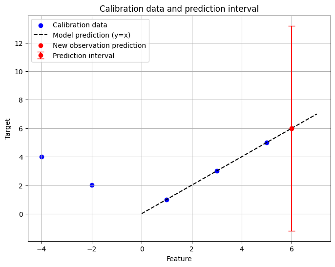
The result is this plot. It displays the calibration data, the model prediction line y=x, the new observation, and its prediction interval—shown as an error bar. In this toy example, note that the calibration data include both positive and negative features; hence the calibration scatter is spread out. The prediction interval is computed accordingly.
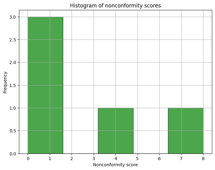
And this other one shows a histogram of the nonconformity scores to illustrate the error distribution.
Why does anyone need dynamic calibration?
Because market conditions change rapidly. It’s essential that the calibration set reflects the most recent market behavior. Here’s a closer look at what dynamic calibration means in this context:
The idea is simple: maintain a calibration set that includes only the most recent N data points. As new data arrive, older observations are discarded. This “sliding window” ensures that the prediction intervals are computed using data that best represent the current market state.
Each time new data are added, the model’s predictions are re-evaluated and the nonconformity scores—i.e., the absolute differences between the actual and predicted values—are recalculated. This constant updating is crucial for capturing sudden changes in market volatility.
The quantile q used for constructing the interval is recalculated every time the calibration set is updated. This ensures that the width of the prediction interval dynamically adapts to the latest level of error variability.
This dynamic approach helps trading algorithms remain agile and responsive to market turbulence.
