[WITH CODE] Exectuion: Optimal execution strategy

Almgren–Chriss framework to balances the trade-off between expected execution cost and risk

---

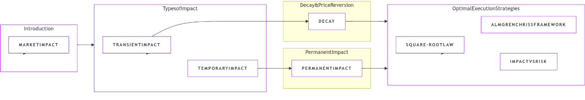
Table of contents:

1. Introduction.

2. Types of impact.

   1. Transient impact.

   2. Temporary impact.

   3. Decay and price reversion.

   4. Permanent impact.

3. The square-root law of market impact.

4. Optimal execution strategies.

   1. The Almgren–Chriss framework.

   2. Impact vs risk.

---

Introduction

Picture this: You’re a master thief planning the ultimate heist. Your target? A vault overflowing with liquid assets—literally. But here’s the twist: the vault is rigged with motion sensors. Make too big a move, and alarms blare, guards swarm, and your grand plan crumbles. Welcome to the world of market impact, where every trade is a high-stakes caper, and the difference between success and disaster is measured in milliseconds and micro-pennies.

Market impact is the phenomenon whereby executing a trade—especially a large one—causes a shift in the price of an asset. For institutional and high‐frequency traders alike, understanding market impact is crucial, as even small changes in execution prices can lead to significant costs.

Let’s dissect it into its various phases.

Types of impact

While small orders often go unnoticed, large orders can disrupt the order book and cause significant price shifts. This phenomenon is crucial for institutional traders and execution algorithms because it directly affects trading costs and execution quality.

Transient impact

It is the immediate, short-lived change in the asset’s price that occurs when a large order is executed. When a large order—e.g., a big guy—is submitted, it "eats" through the visible liquidity on the order book—consuming the shares available at the best prices. As a result, the best bid or ask shifts instantaneously to the next available level. This instantaneous shift is what we call the transient impact.

Consider an order book represented by a cumulative liquidity function, L(p), which indicates the total available volume up to a price p. When a buy order of size Q is placed, the new best ask P_new​ is determined by the smallest price such that:

\(L(P_{\text{new}}) \ge Q\)

The transient impact I_T​ is then given by:

\(I_T = P_{\text{new}} - P_{\text{current}}\)

where P_current​ is the best ask price before the order.

For example, the best ask is $100 with 80 shares available, and the next price level is $100.20 with 120 shares available. If a buy order for 100 shares is executed, the order will completely consume the 80 shares at $100 and then partially take from the next level. Thus, the new best ask will shift to $100.20. The transient impact is:

\(I_T = 100.20 - 100.00 = 0.20 \, (\text{or } 20 \text{ cents})\)

If we represent this, we would have something like this:

Here we see a simulation of a large buy order consuming liquidity, resulting in an immediate upward shift in the best ask.

Temporary impact

It represents the peak reaction that follows the transient impact. Once the large order has been executed and the immediate liquidity consumed, other market participants rapidly adjust their orders. This results in a short-term spike in volatility as the market "overreacts" to the initial shock.

Some stylized facts are:

• Volatility spike: The price overshoots the new equilibrium due to aggressive quoting.

• Peak response: The temporary phase is marked by the highest price deviation.

• Short duration: Typically lasts only for a brief period before the market starts to revert.

This can be modeled by adding an additional component, ΔI, to the transient impact:

\(I_{\text{temp}} = I_T + \Delta I\)

where:

• I_T​ is the transient impact.

• ΔI captures the extra impact from the market’s overreaction.

Following the earlier scenario, after the transient impact pushes the best ask from $100.00 to $100.20, market participants might react by further adjusting their quotes. This additional reaction, ΔI, may cause the price to momentarily spike even higher before starting to settle down.

The temporary impact reflects the maximum observed price change before the decay phase begins. This is a classic:

Decay and price reversion

After the temporary impact, the market gradually absorbs the shock and reverts toward a new equilibrium. This phase is known as the decay or price reversion phase. It occurs as liquidity providers re-enter the market, and the price correction follows an exponential decay pattern.

The decay of market impact is often modeled using an exponential decay function:

\(I(t) = I_{\text{peak}} \cdot e^{-\frac{t-t_0}{\tau}}\)

where:

• I_peak is the peak impact—typically the temporary impact level.

• t_o​ is the time at which decay begins—end of the temporary phase.

• τ is the decay constant that determines the rate at which the impact dissipates.

As time t increases, the e term​ decreases, and the impact I(t) approaches the permanent level. An example of that:

Permanent impact

It is the lasting price change that persists after all temporary effects have dissipated. It reflects the market’s long-term revaluation following the large order and is considered the new “point of control” level.

We can define it as:

\(I_{\text{perm}} = \lim_{t \to \infty} \left[P(t) - P(0)\right]\)

This limit represents the sustained shift in price that is not undone by the subsequent reversion process.

If after a large buy order the price eventually settles at a level that is higher than the pre-trade price, the difference is the permanent impact. For instance, if the best ask moves from $100 to a new stable level of $100.05 after the market absorbs the order, the permanent impact is $0.05.

Permanent impact is typically smaller than the initial transient or temporary impacts because some of the immediate price movement is only a short-term reaction. This is a pattern that all chartist cry when they see it:

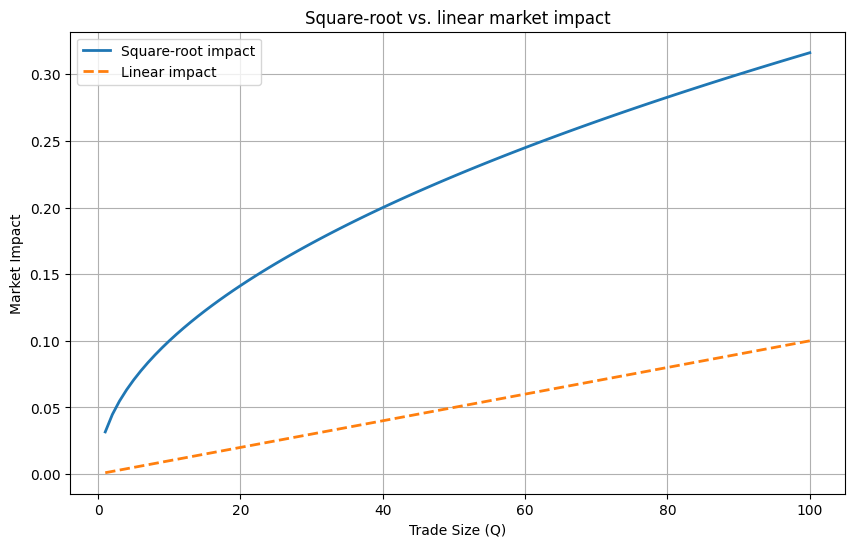
The square-root law of market impact

It is an empirically validated relationship that approximates how much a trade will move the market. It is expressed as:

\(VMI \propto \sigma \cdot \sqrt{\frac{Q}{V}}\)

where:

• MI is the market impact—the change in price caused by the trade.

• σ is the volatility of the asset.

• Q is the trade size.

• V is the daily trading volume.

Market impact increases in a sublinear fashion. This means that if you double the trade size Q, the impact increases only by a factor of √2—approximately 1.41—not by 2.

For large institutional orders, this relationship explains why it’s advantageous to slice orders into smaller parts. Instead of executing a massive order at once—which would dramatically move the price—the order can be divided into smaller chunks, each incurring a smaller impact. Over many chunks, the overall cost is reduced relative to executing the entire order in one go.

The impact is quite different:

Volatility (σ) acts as a multiplier in the formula:

• In volatile markets, prices are more sensitive to trading activity. Even relatively small orders may result in noticeable price changes because σ is higher.

• In calmer markets, the same trade size Q will produce a lower market impact because σ is lower.

This makes the square-root law particularly dynamic: it adjusts the expected impact based on current market conditions.

So why the square-root law is useful?

• To estimate the cost of executing a trade. By knowing the expected impact, a trader can decide whether to proceed with the order as planned or adjust the execution strategy.

• Because impact scales sublinearly, large orders are typically broken into smaller ones to get optimal execution.

• To optimize the sequence of order placement—smart order routing.

Read more about it in this PDF:

Direct Estimation of Equity Market Impact

252KB ∙ PDF file

Download

Download

Optimal execution strategies

Optimal execution strategies aim to split a large order into smaller pieces to minimize total execution costs. These costs stem from two primary sources: the market impact incurred by executing trades—both temporary and permanent—and the risk associated with holding an inventory while the market moves. The challenge is to find the right balance between minimizing impact costs and reducing the risk from price volatility.

One popular model in this domain is the Almgren–Chriss framework, which balances the trade-off between expected execution cost and risk.

The Almgren–Chriss framework

In the discrete-time Almgren–Chriss model, an investor needs to sell X shares over N intervals. Let v_k​ denote the shares traded in period k, and let the execution price be modeled as:

\(p_k = p_{k-1} + \theta v_k + \varepsilon_k\)

where θ represents the permanent impact coefficient and ε_k​ is an IID noise term. The effective execution price incorporates temporary impact and is given by:

\(\tilde{p}_k = p_k + \rho v_k + \frac{S}{2}\,\text{sgn}(v_k),\)

with ρ as the temporary impact coefficient and S the bid–ask spread.

The objective is to minimize the implementation shortfall:

\(C(v) = \sum_{k=1}^{N} v_k \tilde{p}_k - X p_0.\)

This minimization is performed under the constraint:

\(\sum_{k=1}^{N} v_k = X\)

Below is an illustrative Python snippet that uses a simplified version of the optimal execution strategy.

import numpy as np
import matplotlib.pyplot as plt

# Parameters for optimal execution
X = 10000         # total shares to sell
N = 50            # number of trading intervals
p0 = 100.0        # initial price in dollars
theta = 0.0001    # permanent impact coefficient
rho = 0.0002      # temporary impact coefficient
spread = 0.05     # bid-ask spread in dollars

# Time grid
time_grid = np.linspace(0, 1, N+1)

# Assume a constant trading schedule (VWAP strategy)
v_optimal = X / N * np.ones(N)

# Compute the evolution of the asset position
X_remaining = [X]
price = [p0]
for v in v_optimal:
    # Update price due to permanent impact (simplified)
    new_price = price[-1] + theta * v
    price.append(new_price)
    X_remaining.append(X_remaining[-1] - v)

For the purpose of this example, we assume a constant trading rate—by using the VWAP—and plot the evolution of the remaining shares over time.

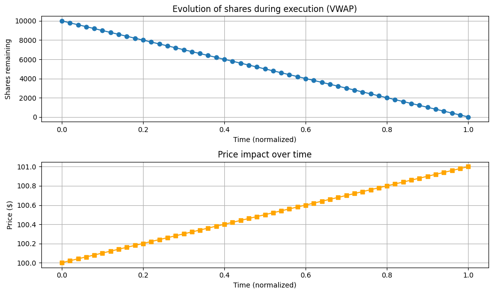
This shows how a constant trading rate reduces the position gradually and how the permanent impact causes a slow drift in the price. More advanced optimal execution algorithms would incorporate risk aversion and adjust the trading schedule accordingly.

Impact vs risk

In many models—such as the Almgren–Chriss framework—the cost function is formulated as a sum of two components:

• Expected impact cost: This is often modeled as a function of the trading rate. For instance, a temporary impact cost might be quadratic in the number of shares traded during each time interval.

• Risk cost: This reflects the uncertainty due to holding inventory over time. The risk cost is typically modeled as proportional to the squared remaining inventory—which, in turn, depends on the volatility of the asset.

A common objective is:

\(\min_{\{v_k\}} \quad \mathbb{E}[C(v)] + \lambda\, \text{Var}[C(v)]\)

subject to

\(\sum_{k=1}^N v_k = X,\)

where:

• v_k​ is the number of shares traded in the kth interval.

• X is the total number of shares to execute.

• λ is the risk aversion parameter.

• E[C(v)] represents the expected execution cost.

• Var[C(v)] captures the risk, which is typically linked to the remaining inventory.

The following Python snippet shows a discrete-time optimal execution problem. Here, we assume:

• The temporary impact cost is quadratic in the trade size:

  \(\theta \, v_k^2\)

• The risk cost is proportional to the squared remaining inventory over each interval, scaled by the volatility σ and risk aversion λ.

The remaining inventory at time step k is computed as the total order X minus the cumulative sum of executed shares. The overall objective is then the sum of the impact cost and risk cost.

import numpy as np
from scipy.optimize import minimize

def cost_function(v, X, theta, sigma, lambda_risk, dt):
    """
    Objective function combining temporary impact cost and risk cost.
    
    Parameters:
      v : array-like, trades in each interval (length N)
      X : total shares to execute
      theta : temporary impact coefficient
      sigma : volatility (affects risk)
      lambda_risk : risk aversion parameter
      dt : length of each time interval
      
    Returns:
      Total cost = impact cost + risk cost.
    """
    # Compute remaining inventory: start with X and subtract cumulative executed shares.
    X_remaining = np.concatenate(([X], X - np.cumsum(v)))
    
    # Impact cost: sum of theta * v^2 over each interval.
    impact_cost = np.sum(theta * v**2)
    
    # Risk cost: proportional to the squared remaining inventory.
    # We sum over intervals (ignoring the final term since inventory is zero by design).
    risk_cost = lambda_risk * sigma**2 * np.sum(X_remaining[:-1]**2 * dt)
    
    return impact_cost + risk_cost

# Example parameters for the execution problem.
X = 10000.0         # Total shares to sell
N = 50              # Number of trading intervals
theta = 0.0001      # Temporary impact coefficient
sigma = 0.02        # Volatility per unit time
lambda_risk = 0.1   # Risk aversion parameter
dt = 1.0 / N        # Assume total execution time is normalized to 1

# Initial guess: Uniform trading (VWAP strategy)
v0 = np.ones(N) * (X / N)

# Constraint: Total shares executed must equal X.
constraints = {'type': 'eq', 'fun': lambda v: np.sum(v) - X}

# Bounds: Assume nonnegative trades (no short selling).
bounds = [(0, X) for _ in range(N)]

# Solve the optimization problem.
result = minimize(cost_function, v0, args=(X, theta, sigma, lambda_risk, dt),
                  constraints=constraints, bounds=bounds, method='SLSQP', options={'disp': True})

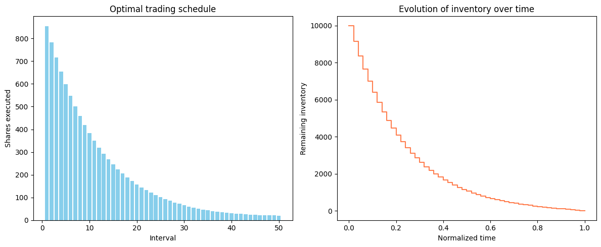
optimal_schedule = result.x

# Compute remaining inventory for plotting.
X_remaining = np.concatenate(([X], X - np.cumsum(optimal_schedule)))

The optimizer finds a schedule that reduces the temporary impact by avoiding overly aggressive trading while also lowering risk by depleting the inventory faster in a volatile environment. On the other hand, increasing the risk aversion parameter λ_risk​​ would tend to front-load the trades, thereby reducing the time the investor is exposed to price risk.

After calibrating the market impact model parameters, the next step is to integrate these into the execution algorithm. This pipeline needs:

• To stimate parameters such as volatility σ, temporary impact coefficient θ, permanent impact coefficient, and other constants.

• Determining the optimal trading schedule that minimizes execution cost and risk.

So let’s build the whole process:

import numpy as np
from scipy.optimize import minimize
import matplotlib.pyplot as plt
import logging

# Set up logging for debugging and informational messages.
logging.basicConfig(level=logging.INFO, format='%(levelname)s: %(message)s')

def calibrate_parameters():
    """
    Placeholder calibration function.
    In practice, these parameters are estimated from historical order book and trade data.
    
    Returns:
        sigma (float): Volatility (per unit time).
        theta (float): Temporary impact coefficient.
        rho (float): Impact related to liquidity consumption.
        tau (float): Decay constant for temporary impact (not used in this discrete example).
        Y (float): Constant from the square-root law.
    """
    sigma = 0.02      # Volatility (e.g., daily or per-unit-time volatility)
    theta = 0.0001    # Temporary impact coefficient
    rho = 0.0002      # Impact related to liquidity consumption (if used separately)
    tau = 10.0        # Decay constant for temporary impact (not used in this discrete example)
    Y = 1.0           # Constant from the square-root law (for larger-scale impact estimation)
    return sigma, theta, rho, tau, Y

def cost_function(v, X, theta, sigma, lambda_risk, dt):
    """
    Combined cost function: temporary impact cost + risk cost.
    
    Parameters:
        v (np.array): Trades in each interval (length N).
        X (float): Total shares to execute.
        theta (float): Temporary impact coefficient.
        sigma (float): Volatility (affects risk).
        lambda_risk (float): Risk aversion parameter.
        dt (float): Length of each time interval.
        
    Returns:
        float: Total execution cost.
    """
    # Compute remaining inventory: initial X minus cumulative executed shares.
    X_remaining = np.concatenate(([X], X - np.cumsum(v)))
    # Temporary impact cost (quadratic cost).
    impact_cost = np.sum(theta * v**2)
    # Risk cost: proportional to squared remaining inventory over time.
    risk_cost = lambda_risk * sigma**2 * np.sum(X_remaining[:-1]**2 * dt)
    return impact_cost + risk_cost

def optimize_schedule(X, N, theta, sigma, lambda_risk, dt):
    """
    Optimize the trading schedule by minimizing the combined cost function.
    
    Parameters:
        X (float): Total shares to execute.
        N (int): Number of trading intervals.
        theta (float): Temporary impact coefficient.
        sigma (float): Volatility.
        lambda_risk (float): Risk aversion parameter.
        dt (float): Normalized time step.
        
    Returns:
        np.array: Optimal trading schedule (shares per interval).
    """
    def cost_func(v):
        return cost_function(v, X, theta, sigma, lambda_risk, dt)
    
    # Initial guess: Uniform trading (VWAP strategy).
    v0 = np.ones(N) * (X / N)
    constraints = {'type': 'eq', 'fun': lambda v: np.sum(v) - X}
    bounds = [(0, X) for _ in range(N)]
    
    result = minimize(cost_func, v0, method='SLSQP', constraints=constraints, bounds=bounds, options={'disp': False})
    if not result.success:
        logging.error("Optimization failed: %s", result.message)
    return result.x

def simulate_execution(opt_schedule, S0, theta, rho, sigma, dt):
    """
    Simulate a price path during execution.
    
    Each trade contributes to:
      - A permanent impact: cumulative effect from executed trades.
      - An instantaneous temporary impact.
      - A stochastic noise term modeling market volatility.
    
    Parameters:
        opt_schedule (np.array): Optimal trading schedule (shares per interval).
        S0 (float): Initial price.
        theta (float): Permanent impact coefficient.
        rho (float): Temporary impact coefficient.
        sigma (float): Volatility.
        dt (float): Time interval length.
        
    Returns:
        np.array: Simulated price path.
    """
    N = len(opt_schedule)
    S = np.zeros(N + 1)
    S[0] = S0
    for k in range(N):
        permanent_impact = theta * opt_schedule[k]
        temporary_impact = rho * opt_schedule[k]
        noise = sigma * np.sqrt(dt) * np.random.randn()
        S[k + 1] = S[k] + permanent_impact + temporary_impact + noise
    return S


def main():
    # Set parameters for execution.
    X = 10000.0        # Total shares to execute
    N = 50             # Number of trading intervals
    lambda_risk = 0.1  # Risk aversion parameter
    dt = 1.0 / N       # Normalized time step
    S0 = 100.0         # Initial price
    
    # Calibrate model parameters.
    sigma, theta, rho, tau, Y = calibrate_parameters()
    logging.info("Calibrated parameters: sigma=%.4f, theta=%.4f, rho=%.4f, tau=%.2f, Y=%.2f", sigma, theta, rho, tau, Y)
    
    # Optimize trading schedule.
    optimal_schedule = optimize_schedule(X, N, theta, sigma, lambda_risk, dt)
    logging.info("Optimal trading schedule computed.")
    
    # Compute remaining inventory.
    inventory = np.concatenate(([X], X - np.cumsum(optimal_schedule)))
    
    # Simulate execution price path.
    price_path = simulate_execution(optimal_schedule, S0, theta, rho, sigma, dt)
    
    # Calculate optimal total cost.
    total_cost = cost_function(optimal_schedule, X, theta, sigma, lambda_risk, dt)
    
    # Print summary results.
    print("Optimal Trading Schedule (shares per interval):\n", optimal_schedule)
    print("Final Simulated Price:", price_path[-1])
    print("Optimal Total Execution Cost: {:.2f}".format(total_cost))

if __name__ == '__main__':
    main()

The output should be something like:

It displays the optimal trading schedule, but you can plot or print the evolution of inventory, the simulated price path, and even some kind of statistics.

Okay everybody! That wraps it up for now! Until next time—stay curious, trade smart, and let the numbers lead the way! 💹

PS: Do you foresee more democratized access to institutional-grade tools for retail algos?

---

👍 Who do you know who is interested in quantitative finance and investing?

---

Appendix

Here a lecture about market impact an large trades

Market impact of large trades and optimal execution

7.94MB ∙ PDF file

Download

Download