

[WITH CODE] Risk Engine: Circuit breaker
Adaptive p-values, a new frontier in algorithmic trading

Table of contents:
Introduction.
Intrinsic risks within unconstrained automation.
Dynamic Circuit Breaker architecture
False Discovery Rate control.
Adaptive window size mechanism.
The Decay-LORD algorithm for FDR control.
Meta-learning framework
Algorithmic implementation.
PnL stream characterization through adaptive P-Values.
FDR control for anomaly thresholding.
Extracting circuit signals: Meta-features.
The Meta-Model's intuition engine.
Circuit breaker state management and rules.
Online decay calibration.
Before you begin, remember that you have an index with the newsletter content organized by clicking on “Read full story” in this image.

Introduction
Once the buy or sell order is opened, success and catastrophe often balance on a knife's edge. Imagine your meticulously crafted trading algorithm humming along, generating steady profits across diverse market conditions. Then suddenly—perhaps triggered by an unexpected geopolitical event or market regime shift—your algorithm begins hemorrhaging capital at an alarming rate. By the time human intervention occurs, significant damage has already been done. This scenario isn't hypothetical; it's a recurring nightmare for quantitative traders worldwide.
The fundamental vulnerability lies in the static nature of most trading safeguards. Traditional circuit breakers typically implement rigid thresholds—stop trading if daily losses exceed x%—but markets are dynamic, complex adaptive systems where yesterday's normal volatility might be today's warning sign. These conventional approaches fail to adapt to changing market conditions and frequently lead to suboptimal outcomes: either excessive trading interruptions during benign volatility or insufficient protection during genuine market dislocations:
The implementation of dynamic circuit breakers introduces its own set of risks. False positives can unnecessarily halt profitable strategies during normal market fluctuations, while false negatives might allow catastrophic losses to accumulate. Statistical methods that are too sensitive create operational inefficiencies; those not sensitive enough fail to provide meaningful protection. Furthermore, circuit breakers that rely solely on historical patterns may fail spectacularly during unprecedented market conditions—precisely when protection is most needed.
Do you remember the March 2020 COVID market crash? When numerous algorithmic trading systems continued operating in wildly irregular market conditions, resulting in devastating losses across the quantitative trading industry. This pivotal event highlighted the urgent need for more sophisticated, adaptive circuit breaker mechanisms capable of distinguishing between normal volatility and genuine strategy failure.

Intrinsic risks within unconstrained automation
The risks associated with an unconstrained algorithmic model are multi-faceted and insidious. Beyond simple performance degradation, we face systemic vulnerabilities:
An algorithm's actions can exacerbate market movements, leading to positive feedback loops where selling triggers more selling, accelerating losses beyond recoverable points.
Models trained on historical data can be too sensitive to conditions outside their training distribution, rendering them fragile when faced with truly novel market behavior.
A minor flaw in logic, amplified by the speed and scale of algorithmic execution across multiple markets or assets, can lead to significant, correlated losses.
Rare, high-impact events are, by definition, impossible to predict and model. An algorithm without a general safety mechanism is particularly exposed to these occurrences.
Dynamic Circuit Breaker architecture
Recently, a fellow I met with asked me what circuit breaker I used. Up until today, I've used a fairly effective one, but curiosity got the better of me. So I've been developing new approaches.
Specifically, the one you're about to read about. It's just a prototype, so it's far from production-ready. It requires a fair amount of refinement, but you'll get an idea of what's going on.
The adaptive trading circuit breaker framework falls within the paradigm of algorithmic risk management or RiskOps. Rather than implementing static loss thresholds, this methodology continuously monitors trading performance through statistical lens, dynamically adjusting to changing market conditions.
False Discovery Rate control
The cornerstone of our approach lies in statistical rigor—specifically, controlling the False Discovery Rate (FDR) when identifying anomalous trading losses. Let's formalize this mathematically:
For a profit and loss time series, we compute p-values pt representing the probability of observing a loss at least as extreme as Xt under normal operating conditions.
The null hypothesis H0 represents the scenario where the trading algorithm is functioning correctly, while the alternative hypothesis H1 indicates a trading anomaly requiring intervention.
The FDR is defined as:
Where:
V is the number of false discoveries (incorrectly identified anomalies)
R is the total number of rejections (total identified anomalies)
R∨1=max(R,1)
This approach generates time-varying rejection thresholds αt such that:
Adaptive window size mechanism
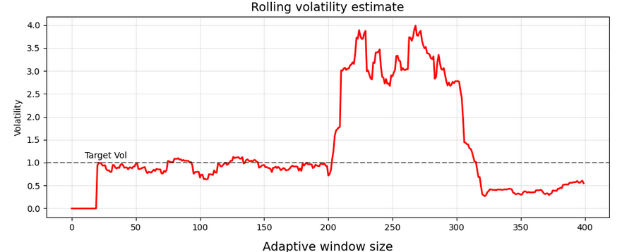
A crucial innovation in this methodology is the dynamic adjustment of the statistical estimation window. Traditional approaches use fixed-size windows, but our framework adapts window size based on observed market volatility:
Where:
wt is the adaptive window size at time t.
wmin and wmax are the minimum and maximum allowed window sizes.
wbase is the baseline window size.
σt is the current volatility estimate.
σtarget is the target volatility level.
This mechanism elegantly addresses a fundamental challenge in statistical estimation. During high volatility periods, larger samples are required to maintain estimation accuracy.

The Decay-LORD algorithm for FDR control
The temporal dimension of trading data introduces unique challenges for statistical testing—recent observations carry more information about current market conditions than distant ones. We implement a modified version of the Decay-LORD algorithm, which incorporates memory decay into FDR control:
Where:
α is the target FDR level
δ is the memory decay parameter
γt=1/t(t+1) represents the sequence of decreasing values.
Rt-L-1 is the set of previous rejections up to time t−L−1.
L is the lag parameter to account for local dependencies.
This formulation elegantly balances the need for statistical rigor with the reality that financial time series exhibit temporal dependence and non-stationarity.
You can check more about FDR control here:

Meta-learning framework
While statistical detection provides a robust foundation, market complexity demands an additional layer of intelligence. Our framework incorporates a lightweight online meta-learning model that analyzes higher-order patterns in the trading data:
Where:
yt indicates anomaly status at time t.
xt represents a feature vector including volatility, skewness, and sign imbalance.
w are model weights updated via online gradient descent.
σ(⋅) is the sigmoid function:
\(\sigma(z) = prob_t = \frac{1}{1+e^{-z}} \)
The weight update rule follows:
Where η is the learning rate. This meta-model complements the statistical approach by incorporating domain-specific features that might indicate trading anomalies even when raw PnL values don't trigger statistical thresholds.

Algorithmic implementation
Moving from the conceptual need to the concrete design, the TradingCircuitBreaker presents a fascinating layered architecture. It’s a system that doesn't just look at the final PnL number, but analyzes its statistical characteristics to make decisions. Think of it not as a simple tripwire, but as an intelligent sensor network constantly assessing the 'health' of the trading process.
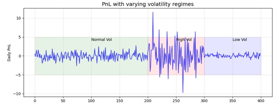
PnL stream characterization through adaptive P-Values
The first thing this circuit breaker needs to do is understand the raw incoming data – the PnL stream. It doesn't just look at the number; it asks, "How unusual is this number right now, given what's happened recently?" To answer that, it calculates a one-sided p-value for each day's PnL, PnLt . A low p-value—close to 0—means, "Wow, seeing a loss this big or bigger is statistically quite rare based on the recent past."
To figure out what's rare, it estimates the average and variability of the PnL over a rolling window. But markets change, right? So, the clever part is that the size of this window isn't fixed. It adapts! If the market gets choppy, the window expands to smooth things out. If things calm down, the window shrinks to react faster to subtle shifts. It's like the system adjusting its focus based on how blurry the picture is.
To calculate these rolling statistics efficiently, especially with a changing window size, the code uses cumulative sums of the PnL and PnL squared. This is just a computational shortcut, letting us quickly grab the sum or sum-of-squares over any recent window.
Once it has the mean and standard deviation for the adaptive window wt, it calculates a Z-score for the current PnLt:
This Z-score tells us how many standard deviations away from the recent mean the current PnL is. Assuming the PnL follows a Normal distribution locally, the one-sided p-value pt is then found using the Normal CDF:
This pt is our core signal, quantifying the surprise of the current PnL relative to the recent, adaptively-defined normal.
Here's the code snippet where this p-value calculation happens:
def compute_pnl_p_values(self, pnl: np.ndarray) -> np.ndarray:
        """
        Estimate one-sided p-values from PnL using adaptive rolling Normal fit.

        Parameters
        ----------
        pnl : np.ndarray
            Time series of profit-and-loss values.

        Returns
        -------
        p_vals : np.ndarray
            P-values indicating probability of observing <= current PnL.
        """
        n = len(pnl)
        p_vals = np.ones(n)
        cs = np.concatenate([[0.], np.cumsum(pnl)])
        cs2 = np.concatenate([[0.], np.cumsum(pnl**2)])
        # global target volatility
        if n > self.target_vol_window:
            s1 = cs[self.target_vol_window]
            s2 = cs2[self.target_vol_window]
            var0 = (s2 - s1**2/self.target_vol_window) / (self.target_vol_window - 1)
            target_vol = math.sqrt(var0) if var0>0 else 1.0
        else:
            target_vol = np.std(pnl)
        for t in range(self.min_window, n):
            # rolling volatility estimate
            wv = min(self.target_vol_window, t)
            s1 = cs[t] - cs[t-wv]
            s2 = cs2[t] - cs2[t-wv]
            var_w = (s2 - s1**2/wv) / (wv-1) if wv>1 else 0.0
            vol = math.sqrt(var_w) if var_w>0 else target_vol
            # adaptive window size
            win = int(self.base_window * (1 + vol/target_vol))
            win = max(self.min_window, min(self.max_window, win, t))
            # compute normal fit
            s1 = cs[t] - cs[t-win]
            s2 = cs2[t] - cs2[t-win]
            mu = s1 / win
            var = (s2 - s1**2/win) / (win-1) if win>1 else var_w
            sigma = math.sqrt(var) if var>0 else 1e-8
            z = (pnl[t] - mu) / sigma
            p_vals[t] = 0.5 * (1 + math.erf(z / math.sqrt(2)))
        return p_vals
If you plot the PnL alongside these p-values. You'd visually see how big negative swings cause the p-value line to plummet towards zero, quantifying just how statistically off things are feeling at that moment. This sequence of p-values is the first step in the breaker's decision process.
FDR control for anomaly thresholding
Getting a low p-value is interesting, but if you look every day, you're bound to see low values just by chance sometimes. This is the multiple testing problem. Constantly checking for rare events means you'll get false discoveries. The compute_breaker_thresholds method tackles this using FDR control, specifically tailored for looking at data sequentially. Instead of trying to avoid any false alarms—which is super hard and makes you miss real stuff—FDR control aims to limit the proportion of false alarms among all the times you do signal an anomaly.
It does this by setting a dynamic threshold at for the p-values pt. If pt≤at, we flag it as an FDR anomaly. The clever part? The threshold at isn't static. It adjusts based on a target FDR level α—like saying, "Okay, we accept that up to 10% of our anomaly flags might be false alarms over the long run"—and, crucially, it reacts to past alarms.
The threshold at is calculated iteratively. A core part of its value comes from α. But when an anomaly is detected at some time j, this detection adds a decreasing weight—using a sequence like γi=1/(i(i+1))—to the threshold for future times t>j. So, if you see an anomaly, the system makes it slightly harder to flag the very next point as an anomaly, preventing a chain reaction of false alarms based on one event. The decay parameter and lag L influence how quickly this memory of past rejections fades and which past rejections matter.
The heart of the dynamic threshold calculation is updating at based on α and the influence of previous rejections.
def compute_breaker_thresholds(self, p_values: np.ndarray) -> (np.ndarray, np.ndarray):
        """
        Generate FDR-based circuit breaker thresholds using Decay-LORD.

        Parameters
        ----------
        p_values : np.ndarray
            PnL p-values.

        Returns
        -------
        anomalies : np.ndarray
            Boolean mask of FDR-detected loss anomalies.
        thresholds : np.ndarray
            Threshold levels at each time step.
        """
        n = len(p_values)
        idx = np.arange(1, n+1)
        gamma = 1.0 / (idx * (idx+1.0))
        tilde = np.maximum(gamma, 1.0 - self.decay)
        thresholds = np.zeros(n)
        rejs = []
        for t in range(n):
            a = self.alpha * tilde[t]
            if rejs:
                diffs = t - np.array(rejs)
                valid = diffs > self.L
                if valid.any():
                    a += self.alpha * np.sum(gamma[diffs[valid]-1])
            thresholds[t] = a
            if p_values[t] <= a:
                rejs.append(t)
        anomalies = p_values <= thresholds
        return anomalies, thresholds
This gives us the formal anomalies signal – statistically controlled flags for unusual losses.
Extracting circuit signals: Meta-features
Formal p-values are great, but they only tell part of the story. What if the way the PnL is behaving is changing, even if one single day isn't an extreme statistical outlier? This is where extract_circuit_signals comes in. It pulls out higher-level meta-features that describe the recent shape of the PnL distribution over a fixed window—self.base_window.
Think of these as the circuit breaker's senses, picking up on different aspects of the trading rhythm:
Volatility: How big are the swings? Calculated as the standard deviation of PnL over the window.
Skewness: Is the PnL distribution lop-sided? Negative skew means more frequent small wins but occasional large losses—a classic look for some strategies, but a warning if it deepens unexpectedly. This is based on the third moment of the distribution.
Sign imbalance: Are there more winning days than losing days, or vice versa? This is a simple count.
These features give a more nuanced picture than just the p-value alone. They are computed using efficient rolling calculations over the fixed window. Skewness, for instance, involves calculating the rolling third central moment and standardizing it by the standard deviation cubed.
Let's look at the code for extracting these signals:
def extract_circuit_signals(self, pnl: np.ndarray) -> np.ndarray:
        """
        Compute meta-features used by circuit breaker meta-model:
        volatility, skewness, sign imbalance.

        Parameters
        ----------
        pnl : np.ndarray
            PnL time series.

        Returns
        -------
        feats : np.ndarray
            Array shape (n,3) with meta-features.
        """
        n = len(pnl)
        feats = np.zeros((n,3))
        cs = np.concatenate([[0.], np.cumsum(pnl)])
        cs2 = np.concatenate([[0.], np.cumsum(pnl**2)])
        cs3 = np.concatenate([[0.], np.cumsum(pnl**3)])
        w = self.base_window
        for t in range(w, n):
            # volatility
            s1 = cs[t] - cs[t-w]; s2 = cs2[t] - cs2[t-w]
            var = (s2 - s1**2/w)/(w-1) if w>1 else 0.0
            feats[t,0] = math.sqrt(var) if var>0 else 0.0
            # skewness
            s1 = cs[t] - cs[t-w]; s2 = cs2[t] - cs2[t-w]; s3 = cs3[t] - cs3[t-w]
            mu = s1/w; m2 = (s2 - s1**2/w)/w; m3 = (s3 - 3*mu*s2 + 2*mu**3*w)/w
            feats[t,1] = m3/(m2**1.5) if m2>0 else 0.0
            # sign imbalance
            wins = pnl[t-w:t]
            feats[t,2] = (np.sum(wins>0) - np.sum(wins<0))/w
        return feats
These meta-features over time would show you the PnL's personality evolving – perhaps volatility ticking up before a big drop, or skewness deepening into negative territory. These three values form a vector xt that becomes input to the next stage.
The Meta-Model's intuition engine
he circuit breaker doesn't just rely on the formal statistical flags from FDR. It adds a layer of intuition using a simple online meta-model. This model learns to connect the dots between the meta-features—the PnL's personality—and whether a formal FDR anomaly actually occurred. It's like it develops a nose for trouble signs based on experience.
This meta-model is essentially a logistic regression running online. It takes the meta-features xt and combines them linearly using its current set of learned weights wt-1:
This value zt is then squashed into a probability between 0 and 1 using the sigmoid function. This is the meta-model's belief about the likelihood of an anomaly, given the PnL's recent characteristics.
The model learns by comparing its belief probt to what actually happened—did a formal FDR anomaly anomalies[t] occur?. The error—anomalies[t]−probt—is used to slightly adjust the weights w at each step. This is a simple online learning update, making the model better over time at predicting anomalies from the meta-features.
ef apply_circuit_logic(self, p_values: np.ndarray, anomalies: np.ndarray, features: np.ndarray) -> (np.ndarray, np.ndarray, np.ndarray):
        """
        Combine FDR anomalies and meta-model signals, apply circuit breaker on/off rules.

        Parameters
        ----------
        p_values : np.ndarray
            PnL p-values.
        anomalies : np.ndarray
            Boolean mask from FDR thresholds.
        features : np.ndarray
            Meta-feature matrix.

        Returns
        -------
        status : np.ndarray
            Trading status: 1=ON, 0=OFF.
        meta_w : np.ndarray
            Updated meta-model weights.
        final_anom : np.ndarray
            Combined anomaly mask.
        """
        n = len(p_values)
        if self.meta_w is None:
            self.meta_w = np.zeros(features.shape[1])
        final_anom = anomalies.copy()

        # Ensure meta-model logic only runs when features are available (t >= base_window - 1)
        meta_features_start_idx = self.base_window - 1 if self.base_window > 0 else 0
        if n > meta_features_start_idx: # Only proceed if there's at least one time step with features
            # meta-model online update and signal generation
            for t in range(meta_features_start_idx, n):
                x = features[t]
                z = self.meta_w.dot(x)
                prob = 1/(1+math.exp(-z)) if abs(z)<50 else (1 if z>0 else 0) # Sigmoid
                error = anomalies[t] - prob # Compare prediction to formal FDR anomaly
                self.meta_w += self.meta_lr * error * x # Update meta weights

                # Combine anomaly signals: FDR OR (Meta-model suspects AND negative PnL)
                # Need p_values[t] for this check
                if prob > self.meta_thresh and p_values[t] < 0.5:
                     final_anom[t] = True


        # circuit breaker on/off logic
        status = np.ones(n, dtype=int)
        off_score = -math.log(self.alpha) # Score threshold derived from alpha
        score = 0.0
        on = True
        consec_norm = 0
        for t in range(n):
            # Calculate impact for the current day based on the combined anomaly signal
            # Use max() with a small number to prevent math domain error for log(0) or log(<0)
            # Impact is only from negative PnL surprises (p_values[t] < 0.5)
            imp = -math.log(max(p_values[t], 1e-10)) if final_anom[t] and p_values[t] < 0.5 else 0.0

            score = self.score_decay*score + imp # Update score with decay

            if on:
                if score >= off_score: # Check OFF condition
                    on = False; consec_norm = 0 # Trip OFF
            else: # If currently OFF
                # Count consecutive days without a combined anomaly signal
                consec_norm = consec_norm+1 if not final_anom[t] else 0
                # Check ON conditions
                if consec_norm>=self.on_consec or score<self.min_score:
                    on = True; score = 0.0 # Turn ON, reset score

            status[t] = 1 if on else 0 # Record status for time t
        return status, self.meta_w, final_anom
If this predicted probability probt exceeds a threshold self.meta_thresh AND the PnL for the day was actually negative—pt<0.5—the system flags this day as a combined anomaly final_anom. This means the breaker can be triggered by either a rigorous statistical anomaly OR a pattern the meta-model has learned to associate with trouble, provided PnL was negative. It's the system's intuition getting a vote.
Circuit breaker state management and rules