

Processing: Smoothing algorithms
A roast of fancy algorithms and the shockingly simple truth about machine learning

Table of content:
Introduction.
Particle filter.
Wavelet denoising.
HP filter.
Before you begin, remember that you have an index with the newsletter content organized by clicking on “Read the newsletter index” in this image.

Introduction
Stock prices are like hyper kids at recess: wild, unpredictable, and loud enough to give you a headache. Traditional methods, like simple moving averages, are like that one supervisor who shows up late to the party, only to see the mess after the chaos has already happened.
And then there’s machine learning—oh, machine learning! It’s like that friend who overcomplicates a simple plan. So, the million-dollar question: are ML algorithms better than old-school methods? Well, the answer is: it depends 😇
It depends, particularly on the choice of the ML model and the analytical method used. Now, personally, I’m all about non-directional methods—they’re like the chill yoga instructors of trading. But, by popular demand, I’ll take a look at those three directional ML algorithms.
Particle filters: Think of them as a swarm of cookie-seeking robots, each trying to locate the true cookie jar–the hidden trend–amidst all the chaos.
Wavelet fenoising: This method acts like a LEGO-building microscope that breaks down data into small pieces, cleans out the noise, and reconstructs the signal.
Hodrick-Prescott Filter: Picture a tightrope walker who must maintain balance; the HP filter smooths the trend while keeping close to the original data.
Let’s just say, I’m about to remember why I swiped left on them a long time ago. Aaah! ML and nostalgia... Get ready for some laughs and facepalms—this is gonna be fun!

Let us begin with the first tool, the cookie-seeking robot swarm.
Particle filter
Particle Filters are designed to estimate hidden states in a dynamic system. In our context, the hidden state represents the true underlying stock trend, and the observable measurements are the noisy stock prices.
We start with a state-space model that consists of two equations:
State evolution equation:
The hidden state xt at time t evolves from the previous state xt-1 plus some random fluctuations–think of it as cookie crumbs left behind by sneaky cookie thieves:
where:
Observation equation:
The observed price zt is modeled as the hidden state plus some measurement noise–like wind dispersing the cookie smell:
where vt is modeled by a heavy‑tailed distribution such as the Student’s t‑distribution:
The degrees of freedom df control how heavy the tails are—a low df means extreme events (or extra crunchy cookies) are more likely.
Updating the particle filter:
The Particle Filter approximates the probability distribution of xt using a set of particles
The algorithm follows these steps:
Initialization: Start with N particles distributed according to a prior belief about x0.
Prediction–motion update: For each particle, update its state using the state evolution equation:
Note: For highly non‑stationary situations, the variance is adjusted dynamically.
Update–measurement update: The likelihood for each particle is computed using the Student’s t‑distribution:
and the weights are updated as:
Resampling: When the effective number of particles:
falls below a threshold, resample the particles to focus on the most promising cookie jar locations.
This framework is flexible—it can accommodate time‑varying parameters to handle non‑stationarity, while the heavy‑tailed likelihood makes it robust against extreme market moves.
Note: The implementations we're about to review have quite a few flaws—due to library implementations—so your homework is to find them and come up with a better solution from scratch–although we'll also go over this in future posts 🙂 it’s worthy of a paper.
import numpy as np
import matplotlib.pyplot as plt
from scipy.stats import t
# Introduce non‑stationarity by modulating the sine function amplitude
np.random.seed(2025)
n_steps = 700 # Number of time steps
dt = 1 # Time increment
mu = 0.001 # Drift (optional)
sigma = 0.02 # Volatility
# Generate Brownian motion
dX = mu * dt + sigma * np.random.randn(n_steps) * np.sqrt(dt)
prices = np.cumsum(dX)
# Number of particles (our cookie‑seeking bees)
N_particles = 1000
# Initialize particles around the first observed price
particles = np.random.normal(loc=prices[0], scale=1.0, size=N_particles)
weights = np.ones(N_particles) / N_particles # Uniform initial weights
# Storage for the estimated state
estimated_state = []
# Filter parameters
sigma_process = 0.1 # Standard deviation for process noise
df = 3 # Degrees of freedom for heavy‑tailed Student’s t
sigma_measurement = 1.0 # Scale parameter for measurement noise
for t_idx in range(len(prices)):
# Prediction: Particles evolve via a random walk (process noise)
particles += np.random.normal(0, sigma_process, size=N_particles)
# Update: Compute likelihood using the Student's t‑distribution
likelihoods = t.pdf(prices[t_idx] - particles, df=df, loc=0, scale=sigma_measurement)
# Update weights
weights *= likelihoods
weights += 1.e-300 # Avoid numerical underflow
weights /= np.sum(weights) # Normalize weights
# Estimate the current state (weighted mean of particles)
estimated_state.append(np.sum(particles * weights))
# Resample if effective particle number drops too low
Neff = 1. / np.sum(weights**2)
if Neff < N_particles / 2:
indices = np.random.choice(np.arange(N_particles), size=N_particles, p=weights)
particles = particles[indices]
weights.fill(1.0 / N_particles)
# Plot the results
plt.figure(figsize=(10, 6))
plt.plot(prices, 'r.', label="Prices")
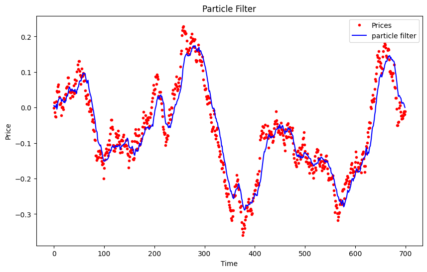
plt.plot(estimated_state, 'b-', label="particle filter")
plt.title("Particle Filter")
plt.xlabel("Time")
plt.ylabel("Price")
plt.legend()
plt.show()The parameters for the example are random, so the output as a directional model leaves much to be desired—being honest, if I had to rate it, it would get a 1/10, and once parameterized, a 5.5/10 💩 sorry guys!
Once parameterized, the Sharpe ratio is <1 and the strategy would be applied:
Let's see if the next one has a higher quality and outperforms this one.
Wavelet denoising
I remember at a dinner, my colleague Mike said:
Wavelet denoising shines when dealing with non‑stationary signals. Unlike the Fourier transform which assumes stationarity, wavelets provide a time‑frequency analysis, breaking data into small blocks that capture both local trends and transient noise.
I don't know what was in that wine, but it was an incredible night. The wavelet approach for non-stationary and heavy-tailed data is built on three pillars:
Decomposition:
The discrete wavelet transform decomposes the signal f(t) into wavelet coefficients:
where ψj,t(t) are wavelet basis functions. This decomposition is ideal for non‑stationary data as it provides localized frequency information.
Thresholding:
Noise (especially if heavy‑tailed) appears as small coefficients in the detail levels. Apply soft thresholding to remove these noisy LEGO pieces:
where θ is a threshold that can be adapted to the data’s variability.
Reconstruction:
Rebuild the signal using the cleaned coefficients:
Let’s implement this model by using the library PyWavelets.
import pywt
# Decompose the non‑stationary signal into wavelet coefficients using 'db4'
coeffs = pywt.wavedec(prices, 'db4', level=3)
# Set a threshold for denoising (this could be made adaptive based on the data)
thresh = 0.5
# Apply soft thresholding to detail coefficients
coeffs[1:] = [pywt.threshold(detail, thresh, mode='soft') for detail in coeffs[1:]]
# Reconstruct the denoised signal from the modified coefficients
denoised_prices = pywt.waverec(coeffs, 'db4')
# Plot the results
plt.figure(figsize=(10, 6))
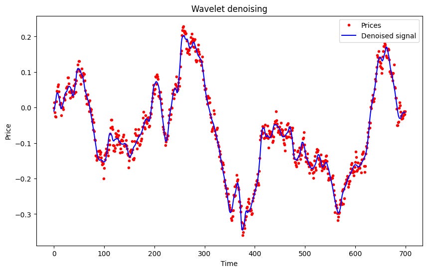
plt.plot(prices, 'r.', label="Prices")
plt.plot(denoised_prices, 'b-', label="Denoised signal")
plt.title("Wavelet denoising")
plt.xlabel("Time")
plt.ylabel("Price")
plt.legend()
plt.show()
Okay, once again, I’ve chosen random parameters. That said, it fits a bit better than the previous filter, but honestly, I doubt it would pass the acid test. It might generate some profit, but with a truly miserable risk-reward ratio.
One flaw you’ll find here is that when a new data point arrives, the coefficients get readjusted during the refit. To avoid this issue, you need to implement an incremental approach. In this [GitHub], you’ll find a carefully curated list of incremental examples—some of them are pure gold!