

AI: LLMs pitfalls
You can summarize the entire article with this question: How many people do you know who have gotten rich using LLMs to produce signal generation and trade? Ok, no more questions.

Table of contents:
Introduction.
The dynamic nature of markets.
The market is a smarter opponent.
Overfitting on historical data.
Finding false positives aka noisy patterns.
Low signal-to-noise ratio.
The algorithmic structure of LLMs.
Before you begin, remember that you have an index with the newsletter content organized by clicking on “Read the newsletter index” in this image.

Introduction
Financial markets are like a never-ending MMA fight where the rules change every 30 seconds, and the referees are all on coffee breaks. It’s a chaotic, ever-evolving battleground where the tiniest edge—like spotting a pattern in the noise or predicting a trend—gets swallowed up faster than a free donut at a trading desk. And here’s the kicker: Large Language Models aka LLMs, despite their jaw-dropping ability to write sonnets about your cat or explain quantum physics in pirate speak, are about as useful in this chaos as a screen door on a submarine.
LLMs like ChatGPT, Deepseek, or Kimi? They’re brilliant at understanding and generating language. They can write you a Shakespearean-level breakup text or explain the history of the stock market in haiku form. But when it comes to predicting financial markets, these models face an insurmountable handicap. They remain fundamentally incapable of competing with established trading benchmarks. They’re out of their depth.
Why? Because markets don’t care about grammar or coherence. They care about patterns—subtle, fleeting, and often nonsensical patterns that even the most advanced LLMs can’t reliably detect. It’s like asking a poet to predict the weather by reading the clouds. Sure, they might get lucky once in a while, but you wouldn’t bet your portfolio on it.

The dynamic nature of markets
The stocks you trade are not the static text of a well-edited book—they’re more like a live, ever-changing conversation where the rules are rewritten at every moment. This dynamic behavior renders any model that relies solely on historical patterns, like LLMs trained on frozen text, fundamentally incapable of predicting future trends or patterns.
We can capture market dynamics with simple, discrete update rules. Consider a trader’s edge that decays over time as competitors catch on. A straightforward model is given by:
where:
Edge(t): The trading advantage at time t.
k: A constant (where 0<k<1) indicating the fraction of the edge lost per time step.
At t=0, the edge is C. With each passing time step, a fixed fraction k of that edge evaporates. This discrete update rule captures the brutal reality that any temporary advantage in trading is fleeting.
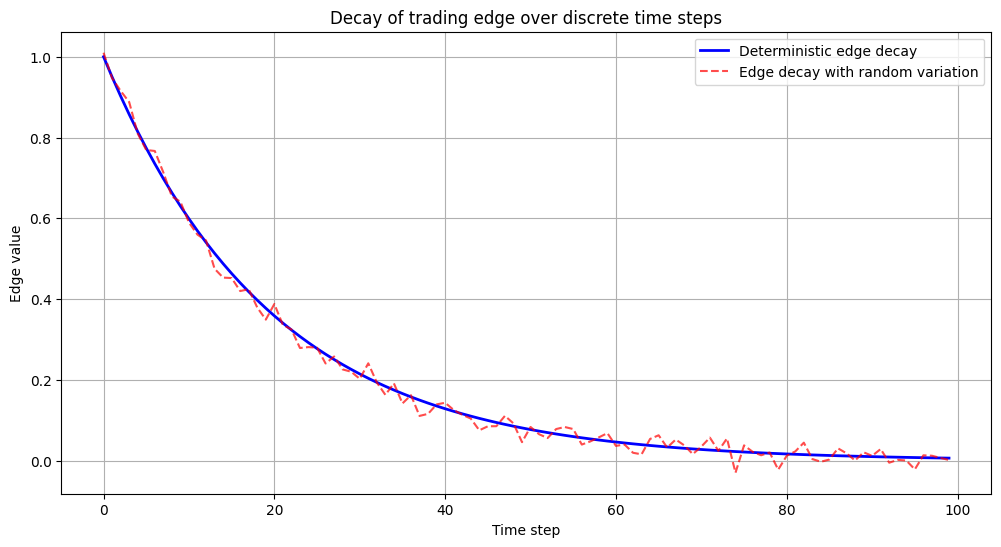
Unless the LLM has found a static true positive over time, using it to predict the market is useless. In the following sections we will look at why and why it will never find a true positive.
Now that we understand how market edges disappear rapidly, we turn to how markets actively fight back.
The market is a smarter opponent
Markets are more than passive archives of past data—they are adaptive adversaries. When a profitable strategy is discovered, the market responds by eroding that advantage as more traders adopt the strategy. This adaptive behavior means that no matter how clever a LLM is at recognizing patterns, it will always be outsmarted by the living, breathing market.
Markets adapt by:
Rapid response to information: When a trading strategy starts generating profits, information about this success rapidly disseminates among market participants—faster than a viral TikTok trend.
Competition and imitation: When a particular approach shows signs of profitability, competitors quickly imitate or even refine the strategy. Even if a new strategy emerges from a novel idea, the moment it is recognized, competition increases dramatically.
Behavioral feedback loops: If many traders start buying a stock based on a certain signal, the resulting price surge might trigger further automated buying, creating a temporary trend. This constant feedback loop ensures that no single strategy can dominate for long.
Technological advancements: The result? It is always a step ahead of any static trading approach.
Sound familiar? Of course it does! So, let’s talk about the one area where LLMs shine: sentiment analysis. But wait—before you start counting your millions, remember: the market is always watching, always adapting 😬
While it is impossible to capture all facets of market adaptation in one equation, a simplified model can illustrate the concept. Consider the following discrete-time update rule that models the adjustment of market sentiment in response to a trading signal:
where:
M(t): Represents the market’s aggregated sentiment or expectation at time t.
I(t): Represents new information or the signal observed at time t.
γ: A learning rate that determines how quickly the market adjusts its sentiment.
In this model, the market’s sentiment M(t) is updated based on the difference between new information I(t) and the current sentiment M(t). The market learns by partially adjusting towards the new information. A higher γ means a faster adaptation, illustrating how quickly market participants can react to new developments.
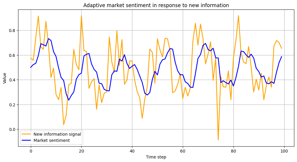
Note that this image is just to illustrate the idea above. But you can imagine what happens when you have a delay in information, resulting in a delay in market entry at a potential edge that lasts minutes or less. In fact, many times the spike from the news is in pre-market so you are late even if you don't want to.
But what about fake news? Are they taken into account when updating the LLMs? If you want to know more, visit the previous post:

Overfitting on historical data
Overfitting is a notorious pitfall in quantitative finance and this is not an exception today. It occurs when a model learns the quirks and noise in historical data rather than the true underlying patterns.
For LLMs, this challenge is even more pronounced because their training data—be it static text, images, or videos—represents historical snapshots that often do not reflect the rapidly evolving, real-time nature of trading environments.
LLMs are designed to predict the next word or token in a sequence, minimizing a loss function such as:
Here, θ represents the model parameters, and wi are the tokens in the training data. While this objective works exceptionally well for language tasks, the same principle lead to overfitting when applied to other domains like time series—this part is directly connected to the final section, it is the last step to make an LLM work. All the effort, all the work itself is absurd..
Time series are not sequential and although they show dependency relationships between values, there is no logical relationship.
When LLMs are fine-tuned on historical financial data, they learn the specific noise inherent in that data—such as market anomalies, one-off events, or artifacts of the data collection process—rather than robust patterns that are predictive of future behavior. Ah! By the way, adding the RL framework only makes things worse.
Why LLMs struggle with overfitting in trading?
The sequential approach.
The non-stationary data.
Overemphasis on patterns that are noise.
Overfitting illustrates a fundamental problem with relying on historical patterns—a problem that plagues LLMs and ML in general.
Finding false positives aka noisy patterns
Finding patterns in a cloud of noise is what all quants call data snooping. It is the practice of exhaustively searching through historical data to find statistically significant patterns.
In a market where randomness reigns, even the most spurious correlations can appear significant if enough tests are performed. You know, data snooping is like rummaging through an enormous junk drawer—if you look long enough, you're bound to find something that seems interesting, even if it's just an old, tangled shoelace.
This means testing thousands of hypotheses until you stumble upon a significant pattern that’s nothing more than random noise.
When you perform many tests on random data, the chance of finding a false positive increases dramatically. Mathematically, if you test N independent hypotheses at a significance level α, the probability of finding at least one false positive is:
For example, if α=0.05 and N=1000, you’d expect nearly all tests to eventually yield a significant result just by chance. It’s like finding a golden ticket in a candy bar—if you buy enough bars, eventually one is bound to say “Congratulations,” even if it’s not really golden. Check it, I use a Laplace distribution for the sake of this example, but you can test it with any distribution you want:
import numpy as np
import matplotlib.pyplot as plt
from scipy.stats import pearsonr

# Parameters
N_tests = 1000
alpha = 0.05
n_points = 1000  # Number of data points in each test

np.random.seed(42)
data = np.random.laplace(0, 1, n_points) # Test with gumble or normal distributions

# Perform N_tests correlation tests between 'data' and new noise series each time
significant_results = 0
p_values = []

for _ in range(N_tests):
    noise2 = np.random.normal(0, 1, n_points)
    r, p = pearsonr(data, noise2)
    p_values.append(p)
    if p < alpha:
        significant_results += 1

print(f"Number of significant results (p < {alpha}): {significant_results} out of {N_tests}")

# Plot a histogram of the p-values
plt.figure(figsize=(12, 6))
plt.hist(p_values, bins=30, color='skyblue', edgecolor='black')
plt.axvline(alpha, color='red', linestyle='dashed', linewidth=2, label=f'Alpha = {alpha}')
plt.title('Histogram of P-values from random correlation tests')
plt.xlabel('P-value')
plt.ylabel('Frequency')
plt.legend()
plt.grid(True)
plt.show()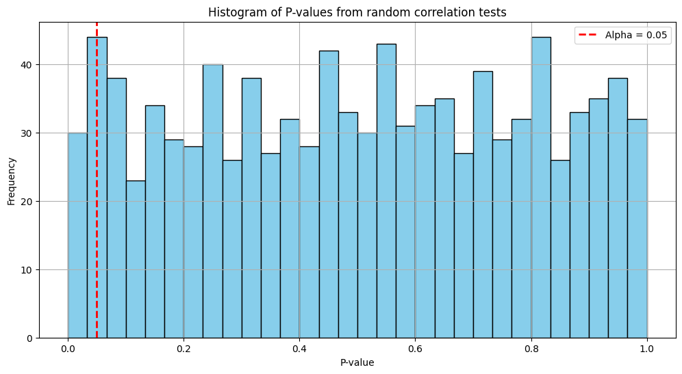
Awesome! The number of significant results (p < 0.05): 50 out of 1000!!! 😮💨
Even though both series are pure noise, around 5% of the tests will show p-values below 0.05 purely by chance. This plot displays the distribution of p-values. Notice how many fall below the significance threshold—proof that if you look hard enough, you can find signals in nothing but noise!
Now that we understand how noise can masquerade as signal, let’s examine why true trading signals are almost always lost in the noise.
Low signal-to-noise ratio
For LLMs built to excel in language processing, the transition to analyzing financial time series is akin to trying to read an invisible ink message in a hurricane. No, wait, are you using them to mine trading data? Don’t tell me… time series!?
Here the dilemma, in financial markets, the observed return rt can be written as:
where the signal is the genuine, predictive information, and the noise is the random, unpredictable fluctuation. For trading data, the standard deviation of the true signal (σSignal) is minuscule compared to that of the noise (σNoise):
LLMs are designed to capture and reproduce complex patterns from vast corpora of static text, where meaningful structures—grammar, context, semantics—are relatively robust. However, the overwhelming noise drowns out these patterns. This means that when an LLM tries to find a signal, it's often just amplifying random fluctuations—mistaking them for genuine market patterns.
The result is a SNR less than 1. This means that the noise in your data is stronger than the actual signal you’re trying to detect. Here are some of the key consequences:
Increased risk of false positives.
Poor predictive performance.
High variability.
Difficulty in parameter estimation.
Imagine an LLM as an overly enthusiastic art critic at a modern art gallery. It sees shapes and patterns in every splatter of paint, convinced that there’s deep meaning behind every random stroke. In the same way, when an LLM analyzes market data