

[WITH CODE] Portfolio: Robust covariance estimation
How to keep your portfolio balanced even when markets misbehave

Table of contents:
Introduction.
Classical approach.
Why the classical approach is called “classical”?
Understanding the Mahalanobis Distance.
Improving computational methods.
An iterative reweighting scheme.
Further than traditional enhancements.
Robust covariance estimation via iterative reweighting.
Shrinkage for additional stability.
Before you begin, remember that you have an index with the newsletter content organized by clicking on “Read full story” in this image.

Introduction
It’s saturday night, you’re at a lively party where everyone has a story to share. Most guests follow a predictable rhythm, but then there’s that one person—loud, unpredictable, and totally off-beat.
In statistics, such a guest is known as an outlier, and its presence can throw off your entire analysis. In traditional quantitative finance and risk management, the covariance matrix plays a starring role. It tells us about the relationships between different assets or variables, much like understanding who at the party pairs well with whom. However, the classical estimation methods, while elegant under ideal conditions, quickly lose their charm when faced with noisy, messy data.
Let’s take a closer look and check if we can enhance this method a little bit.

Classical approach
The concept of the covariance matrix is foundational in portfolio optimization. When dealing with multivariate data—observations that have multiple components or dimensions—understanding how different variables co-vary is critical. This is precisely what the covariance matrix encapsulates: it describes not only how each individual variable spreads out—its variance—but also how each pair of variables co-varies—their covariance.
In a typical scenario, you might have a random vector x∈Rp. This vector has p components, for example, p different stock returns, or p measurements taken on a patient in a clinical trial. The population covariance matrix of x, denoted by Σ, is defined as:
where μ=E[x] is the population mean vector. Of course, in real-world applications, the true mean μ and the true covariance Σ are almost never known. Instead, we collect a sample of observations and use them to estimate these quantities. This is where the classical approach to covariance estimation comes into play.
Suppose we have n observations of the random vector x. We label these observations as x1,x2,…,xn, where each xi∈Rp. The classical sample covariance matrix S is defined by:
with
being the sample mean vector. This definition might look compact, but it encodes several important properties:
Centering by the sample mean: We first subtract the sample mean from each observation. This step ensures that the estimated covariance matrix reflects the variability around the center of the data rather than around an arbitrary origin.
Outer product structure: Each term is a p×p matrix capturing the pairwise product of deviations from the mean for all dimensions. Summing these outer products accumulates information about how variables vary and co-vary.
Division by n−1: Dividing by n−1 (rather than n) is crucial for making S an unbiased estimator of the population covariance Σ. This subtle difference—using n−1 instead of n—comes from Bessel’s correction, a concept that ensures that E[S]=Σ.
Let’s generate some synthetic bivariate data and compute the classical covariance matrix:
import numpy as np

# Generate synthetic data: 100 observations in 2 dimensions
np.random.seed(42)
data = np.random.multivariate_normal([0, 0], [[1, 0.5], [0.5, 1]], size=100)

# Compute the classical covariance matrix
classical_cov = np.cov(data, rowvar=False)
print("Classical Covariance Matrix:")
print(classical_cov)
The classical covariance estimator works beautifully when the data behaves nicely. But financial data is anything but nice data.

Why the classical approach is called “classical”?
This is because it represents the most straightforward and commonly taught estimator in statistics. It also aligns with the maximum likelihood estimator for covariance if we assume the data is drawn from a multivariate normal—Gaussian— distribution. In other words, if we take the log-likelihood of a multivariate normal distribution and differentiate to find the maximum, we arrive at precisely the sample mean and the sample covariance matrix S.
Under these Gaussian assumptions, the sample covariance matrix is optimal in a minimum variance sense. More formally, it is the Best Unbiased Estimator of the covariance when data truly is multivariate normal. This is a strong statement—akin to saying that if the data is well-behaved and indeed follows the normal distribution, you can’t do better than the classical approach in terms of variance of your estimates.
Although, honestly, I would take him classic for its pitfalls:
Sensitivity to outliers.
Breakdown point.
Assumption of Gaussianity.
Numerical instability.
Overfitting in high dimensions.
Inadequate scaling and misleading geometry.
The perfect cocktail to make you lose money. Is there possibly an alternative? Let's see.
Understanding the Mahalanobis Distance
The Mahalanobis distance offers a way to measure how far a point is from a distribution while considering the data’s spread and correlations. For a data point x, its distance from the mean μ is given by
This measure is inherently scale invariant and correlation sensitive, meaning it adjusts the notion of distance based on how the data varies along different directions. In an ideal world, points at the same Mahalanobis distance would lie on ellipsoids centered at μ.
We compute the Mahalanobis distance for a new point like this:
from numpy.linalg import inv

# Compute the mean of the data
mean_vector = np.mean(data, axis=0)

# Inverse of the covariance matrix
cov_inv = inv(classical_cov)

# Define a new data point
x_new = np.array([1, 1])

# Compute Mahalanobis distance
diff = x_new - mean_vector
mahalanobis_distance = np.sqrt(np.dot(np.dot(diff.T, cov_inv), diff))
print("Mahalanobis Distance for x_new:", mahalanobis_distance)
While this method is powerful, it relies entirely on the accuracy of the covariance matrix. If the covariance matrix is distorted by outliers, then the Mahalanobis distance, too, will be misleading—imagine trying to measure the distance in a funhouse mirror!
Improving computational methods
Given the shortcomings of classical approaches, robust covariance estimation methods come to the rescue. These methods aim to downweight or even exclude outliers, leading to a more faithful representation of the central data structure.
At the heart of many robust estimators is an iterative process that adjusts weights for each observation based on how unusual they are. One common approach is to solve an optimization problem of the form
where ρ is a loss function that reduces the impact of observations with large residuals—or high Mahalanobis distances. The Huber loss, for example, behaves quadratically for small deviations and linearly for large deviations, effectively clipping the influence of outliers.
Another popular method is the Minimum Covariance Determinant estimator, which searches for the subset of the data that yields the smallest determinant for the covariance matrix. In other words, it finds the most compact set of observations and uses them to estimate the covariance, thereby sidestepping outliers. Check more about it here:
An iterative reweighting scheme
One way to implement robustness is via an iterative reweighting algorithm. The process is straightforward:
Initialization: Start with the classical estimates for the mean μ(0) and covariance Σ(0).
Compute distances: Calculate the squared Mahalanobis distances for each observation:
\(d_i^2 = (\mathbf{x}_i - \boldsymbol{\mu}^{(k)})^T (\boldsymbol{\Sigma}^{(k)})^{-1} (\mathbf{x}_i - \boldsymbol{\mu}^{(k)}).\)Assign weights: Use a weight function that downscales observations with large distances. For example, a simple rule could be:
\(w_i = \min\left(1, \frac{c}{d_i}\right),\)where c is a chosen cutoff constant.
Update estimates: Update the mean and covariance using these weights:
\(\boldsymbol{\mu}^{(k+1)} = \frac{\sum_{i=1}^{n} w_i \mathbf{x}_i}{\sum_{i=1}^{n} w_i},\)\(\boldsymbol{\Sigma}^{(k+1)} = \frac{\sum_{i=1}^{n} w_i (\mathbf{x}_i - \boldsymbol{\mu}^{(k+1)})(\mathbf{x}_i - \boldsymbol{\mu}^{(k+1)})^T}{\sum_{i=1}^{n} w_i}.\)Iterate: Continue until the estimates converge.
This approach can be thought of as a meticulous party organizer who revisits the guest list repeatedly—removing the disruptive guests (or at least muting their influence) until the party atmosphere is just right.
With a clear understanding of both the pitfalls of classical methods and the potential improvements of robust methods, let’s now see how these ideas translate into code.
import numpy as np
from numpy.linalg import inv, norm
import matplotlib.pyplot as plt
from matplotlib.patches import Ellipse

def robust_covariance(data, c=3.0, max_iter=50, tol=1e-5):
    """
    Compute robust estimates of mean and covariance using an iterative reweighting scheme.

    Parameters:
        data (np.ndarray): Array of observations (n x p).
        c (float): Cutoff constant for weight calculation.
        max_iter (int): Maximum number of iterations.
        tol (float): Tolerance for convergence.

    Returns:
        mu (np.ndarray): Robust estimate of the mean.
        cov (np.ndarray): Robust estimate of the covariance matrix.
    """
    n, p = data.shape

    # Start with classical estimates
    mu = np.mean(data, axis=0)
    cov = np.cov(data, rowvar=False)

    for iteration in range(max_iter):
        # Invert the current covariance estimate
        cov_inv = inv(cov)

        # Compute Mahalanobis distances for each observation
        distances = np.array([np.sqrt(np.dot((x - mu).T, np.dot(cov_inv, (x - mu))))
                              for x in data])

        # Compute weights: downweight observations with large distances
        weights = np.minimum(1, c / (distances + 1e-10))  # small epsilon to avoid division by zero

        # Update the mean estimate
        mu_new = np.sum(weights[:, np.newaxis] * data, axis=0) / np.sum(weights)

        # Update the covariance estimate using weighted deviations
        diff = data - mu_new
        cov_new = np.dot((weights[:, np.newaxis] * diff).T, diff) / np.sum(weights)

        # Check for convergence in both mean and covariance
        if norm(mu_new - mu) < tol and norm(cov_new - cov) < tol:
            print(f"Converged after {iteration + 1} iterations")
            break

        # Update estimates for the next iteration
        mu, cov = mu_new, cov_new

    return mu, cov

# Generate synthetic data: mostly "nice" data with a few outliers
np.random.seed(42)
data_clean = np.random.multivariate_normal([0, 0], [[1, 0.5], [0.5, 1]], size=100)
data_outliers = np.random.multivariate_normal([8, 8], [[1, 0], [0, 1]], size=5)
data_robust = np.vstack([data_clean, data_outliers])

# Compute classical estimates for comparison
classical_mu = np.mean(data_robust, axis=0)
classical_cov = np.cov(data_robust, rowvar=False)

# Compute robust estimates using our iterative algorithm
robust_mu, robust_cov = robust_covariance(data_robust)
print("Robust Mean:", robust_mu)
print("Robust Covariance Matrix:\n", robust_cov)
To fully appreciate the difference, let’s visualize the covariance ellipses for both the classical and robust estimators. The ellipse of a bivariate normal distribution is defined by the equation
where k is a constant that determines the confidence level—typically 2 or 3 standard deviations.
def plot_cov_ellipse(mu, cov, ax, n_std=2.0, edgecolor='black', label=""):
    """
    Plot a covariance ellipse centered at mu, given a covariance matrix.

    Parameters:
        mu (np.ndarray): Center of the ellipse.
        cov (np.ndarray): Covariance matrix.
        ax (matplotlib.axes.Axes): Plotting axis.
        n_std (float): Number of standard deviations for the ellipse radius.
        edgecolor (str): Color of the ellipse edge.
        label (str): Label for the ellipse.
    """
    eigenvals, eigenvecs = np.linalg.eigh(cov)
    order = eigenvals.argsort()[::-1]
    eigenvals, eigenvecs = eigenvals[order], eigenvecs[:, order]

    # Determine the angle of the ellipse (in degrees)
    theta = np.degrees(np.arctan2(*eigenvecs[:, 0][::-1]))
    width, height = 2 * n_std * np.sqrt(eigenvals)

    ellip = Ellipse(xy=mu, width=width, height=height, angle=theta,
                    edgecolor=edgecolor, fc='None', lw=2, label=label)
    ax.add_patch(ellip)

# Create the plot
fig, ax = plt.subplots(figsize=(8, 6))
ax.scatter(data_robust[:, 0], data_robust[:, 1], s=30, label="Data points", alpha=0.6)

# Plot the classical covariance ellipse (red)
plot_cov_ellipse(classical_mu, classical_cov, ax, n_std=2.0, edgecolor='red', label="Classical Covariance")

# Plot the robust covariance ellipse (blue)
plot_cov_ellipse(robust_mu, robust_cov, ax, n_std=2.0, edgecolor='blue', label="Robust Covariance")

ax.set_title("Covariance Ellipses: Classical vs. Robust Estimators")
ax.set_xlabel("X")
ax.set_ylabel("Y")
ax.legend()
plt.show()
And the output is:
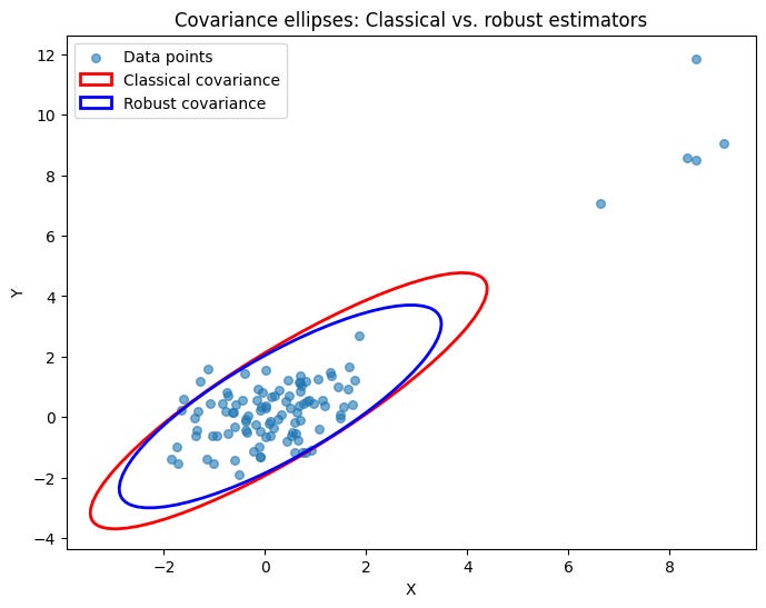
In the resulting plot, you’ll notice that the classical covariance ellipse—in red—tends to stretch towards the outlier points. In contrast, the robust covariance ellipse—in blue—is more centered around the bulk of the data, clearly illustrating how robust methods mitigate the influence of extreme values.
Is this enough? I'm afraid not. Let's look at some improvements I've been working on over time.